Diagnostic Prevalence

Compare PPV or NPV by sensitivity, specificity, and prevalence.

Usage

gg_diagnostic_prev(se, sp, p, result = c("PPV", "NPV"))

gg_prev_fixed(se, sp, p, result = c("PPV", "NPV"), layout = c("lines", "band"))

Arguments

se

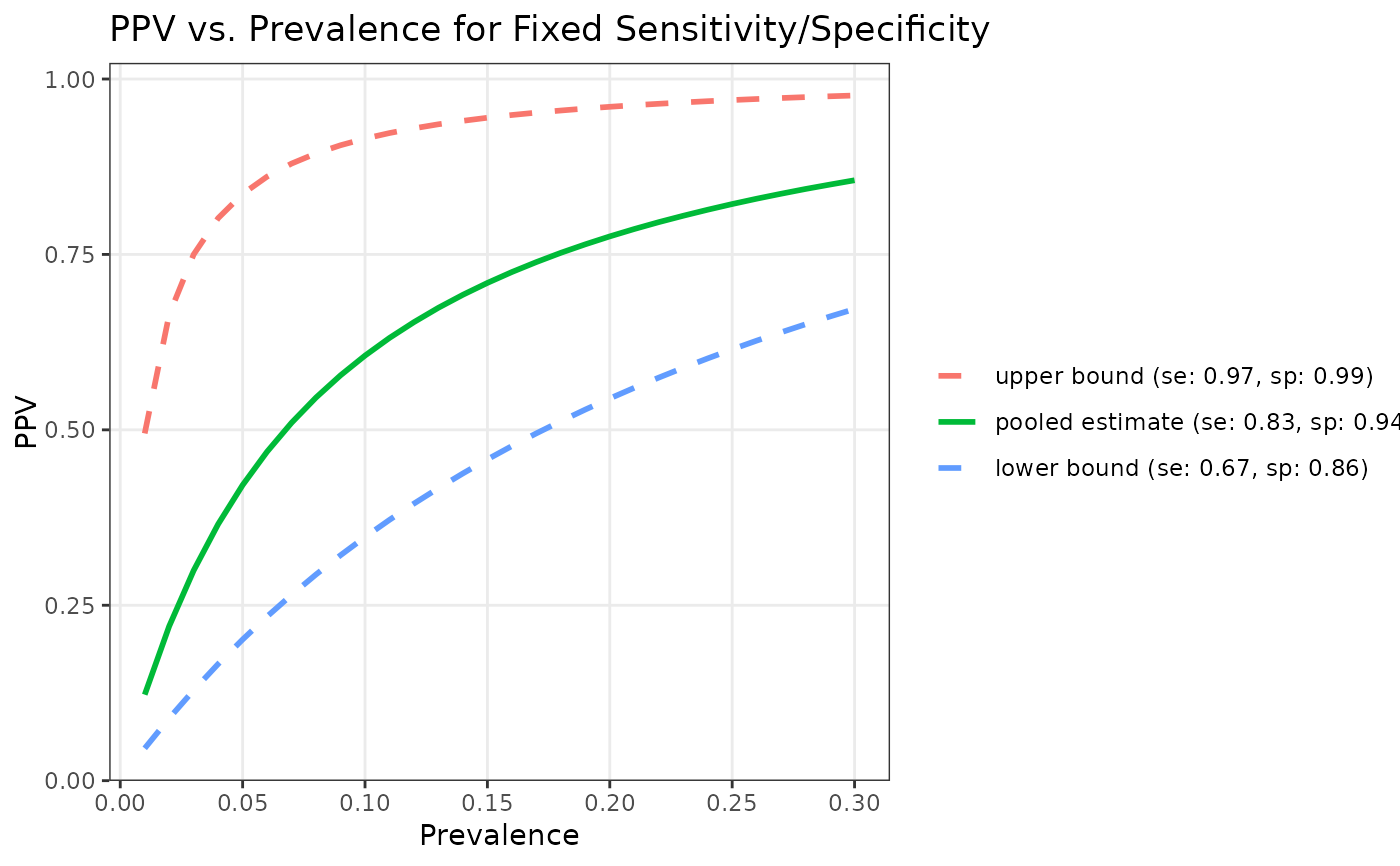
a vector of sensitivity estimates. For gg_prev_fixed, must be a vector of length 3 for lower bound, pooled estimate, and upper bound.

sp

a vector of specificity estimates. For gg_prev_fixed, must be a vector of length 3 for lower bound, pooled estimate, and upper bound. For gg_diagnostic_prev, a sequence of values to plot along x-axis.

p

a vector of prevalence values. For gg_prev_fixed, must be a sequence of values to plot along x-axis.

result

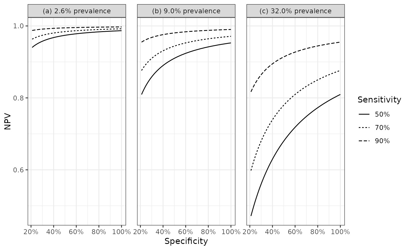
whether to show the PPV or NPV on the y-axis

layout

whether to plot confidence region using "lines" or a filled "band."

Value

Graph of PPV or NPV by specificity, sensitivity, and prevalence.

Details

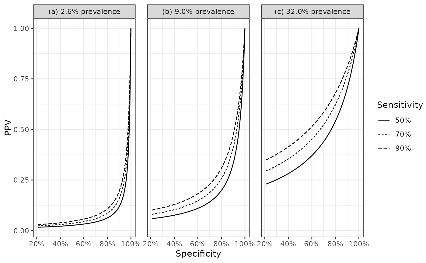
gg_diagnostic_prev plots positive predictive value (PPV) or negative predictive value (NPV) as a function of specificity, with sensitivity separated by line types and prevalence shown across facets.

gg_prev_fixed plots PPV or NPV as a function of prevalence, with coloured lines separating fixed pairs of sensitivity and specificity for the lower bound, pooled estimate, and upper bound.

Author

Derek Chiu

Examples

se <- c(0.5, 0.7, 0.9)
sp <- seq(0.21, 1, 0.01)
p <- c(0.32, 0.09, 0.026)
gg_diagnostic_prev(se, sp, p, result = "PPV")

gg_diagnostic_prev(se, sp, p, result = "NPV")


gg_prev_fixed(
  se = c(0.67, 0.83, 0.97),
  sp = c(0.86, 0.94, 0.99),
  p = seq(0.01, 0.30, 0.01),
  result = "PPV"
)