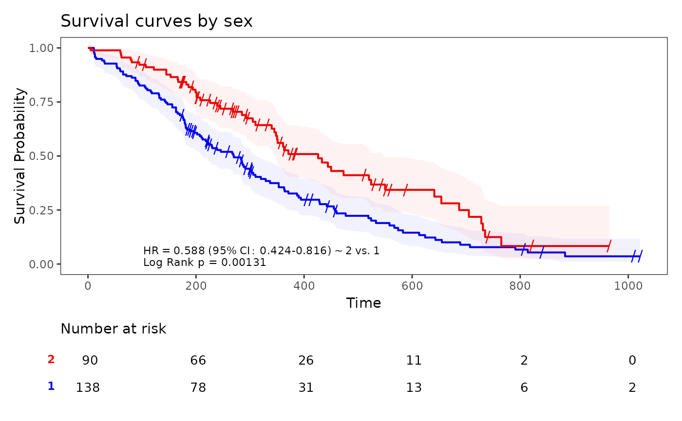
Kaplan-Meier Plots using ggplot — ggkm • biostatUtil

Produce nicely annotated KM plots using ggplot style.

Usage

ggkm(
  sfit,
  sfit2 = NULL,
  table = TRUE,
  returns = TRUE,
  marks = TRUE,
  CI = TRUE,
  line.pattern = NULL,
  shading.colors = NULL,
  main = "Kaplan-Meier Plot",
  xlabs = "Time",
  ylabs = "Survival Probability",
  xlims = NULL,
  ylims = NULL,
  ystratalabs = NULL,
  cox.ref.grp = NULL,
  timeby = 5,
  test = c("Log Rank", "Tarone-Ware"),
  pval = TRUE,
  bold_pval = FALSE,
  sig.level = 0.05,
  HR = TRUE,
  hide_hr_labels = FALSE,
  use.firth = 1,
  hide.border = FALSE,
  expand.scale = TRUE,
  legend = FALSE,
  legend.xy = NULL,
  legend.direction = "horizontal",
  line.y.increment = 0.05,
  size.plot = 11,
  size.summary = 3,
  size.table = 3.5,
  size.table.labels = 11,
  digits = 3,
  ...
)

Arguments

sfit: an object of class survfit containing one or more survival curves
sfit2: an (optional) second object of class survfit to compare with sfit
table: logical; if TRUE (default), the numbers at risk at each time of death is shown as a table underneath the plot
returns: logical; if TRUE the plot is returned
marks: logical; if TRUE (default), censoring marks are shown on survival curves
CI: logical; if TRUE (default), confidence bands are drawn for survival curves the using cumulative hazard, or log(survival).
line.pattern: linetype for survival curves
shading.colors: vector of colours for each survival curve
main: plot title
xlabs: horizontal axis label
ylabs: vertical axis label
xlims: horizontal limits for plot
ylims: vertical limits for plot
ystratalabs: labels for the strata being compared in survfit
cox.ref.grp: indicates reference group for the variable of interest in the cox model. this parameter will be ignored if not applicable, e.g. for continuous variable
timeby: length of time between consecutive time points spanning the entire range of follow-up. Defaults to 5.
test: type of test. Either "Log Rank" (default) or "Tarone-Ware".
pval: logical; if TRUE (default), the logrank test p-value is shown on the plot
bold_pval: logical; if TRUE, p-values are bolded if statistically significant at sig.level
sig.level: significance level; default 0.05
HR: logical; if TRUE (default), the estimated hazard ratio and its 95% confidence interval will be shown
hide_hr_labels: logical; if TRUE and there are only two strata, the strata labels are hidden from HR summary because there is only contrast being compared
use.firth: Firth's method for Cox regression is used if the percentage of censored cases exceeds use.firth. Setting use.firth = 1 (default) means Firth is never used, and use.firth = -1 means Firth is always used.
hide.border: logical; if TRUE, the upper and right plot borders are not shown.
expand.scale: logical; if TRUE (default), the scales are expanded by 5% so that the data are placed a slight distance away from the axes
legend: logical; if TRUE, the legend is overlaid on the graph (instead of on the side).
legend.xy: named vector specifying the x/y position of the legend
legend.direction: layout of items in legends ("horizontal" (default) or "vertical")
line.y.increment: how much y should be incremented for each line
size.plot: text size of main plot
size.summary: text size of numerical summaries
size.table: text size of risk table
size.table.labels: text size of risk table axis labels
digits: number of digits to round: p-values digits=number of significant digits, HR digits=number of digits after decimal point NOT significant digits
...: additional arguments to other methods

Value

A kaplan-meier plot with optional annotations for hazard ratios, log rank test p-values, and risk table counts for each stratum.

Author

Samuel Leung, Derek Chiu

Examples

library(survival)
sfit <- survfit(Surv(time, status) ~ sex, lung)
ggkm(sfit, timeby = 200, main = "Survival curves by sex")