| Subsampling | Algorithms | Overall | HGSOC | CCOC | ENOC | MUOC | LGSOC |
|---|---|---|---|---|---|---|---|
| none | rf | 0.922 | 0.948 | 0.983 | 0.953 | 0.975 | 0.984 |
| svm | 0.92 | 0.947 | 0.982 | 0.955 | 0.975 | 0.982 | |
| xgb | 0.807 | 0.809 | 0.936 | 0.933 | 0.955 | 0.982 | |
| mr | 0.807 | 0.807 | 0.936 | 0.935 | 0.955 | 0.982 | |
| down | rf | 0.804 | 0.853 | 0.975 | 0.903 | 0.959 | 0.92 |
| svm | 0.793 | 0.833 | 0.973 | 0.884 | 0.969 | 0.928 | |
| xgb | 0.783 | 0.833 | 0.968 | 0.897 | 0.961 | 0.907 | |
| mr | 0.829 | 0.87 | 0.977 | 0.912 | 0.961 | 0.938 | |
| up | rf | 0.928 | 0.955 | 0.983 | 0.959 | 0.979 | 0.982 |
| svm | 0.92 | 0.951 | 0.974 | 0.951 | 0.979 | 0.985 | |
| xgb | 0.928 | 0.959 | 0.982 | 0.96 | 0.974 | 0.982 | |
| mr | 0.891 | 0.924 | 0.976 | 0.949 | 0.966 | 0.967 | |
| smote | rf | 0.921 | 0.955 | 0.98 | 0.953 | 0.97 | 0.984 |
| svm | 0.92 | 0.95 | 0.979 | 0.954 | 0.978 | 0.981 | |
| xgb | 0.923 | 0.955 | 0.98 | 0.955 | 0.971 | 0.984 | |
| mr | 0.897 | 0.931 | 0.979 | 0.951 | 0.967 | 0.967 | |
| hybrid | rf | 0.922 | 0.953 | 0.98 | 0.952 | 0.975 | 0.983 |
| svm | 0.916 | 0.944 | 0.982 | 0.951 | 0.975 | 0.979 | |
| xgb | 0.924 | 0.954 | 0.984 | 0.958 | 0.971 | 0.982 | |
| mr | 0.892 | 0.925 | 0.978 | 0.947 | 0.967 | 0.966 |
4 Results
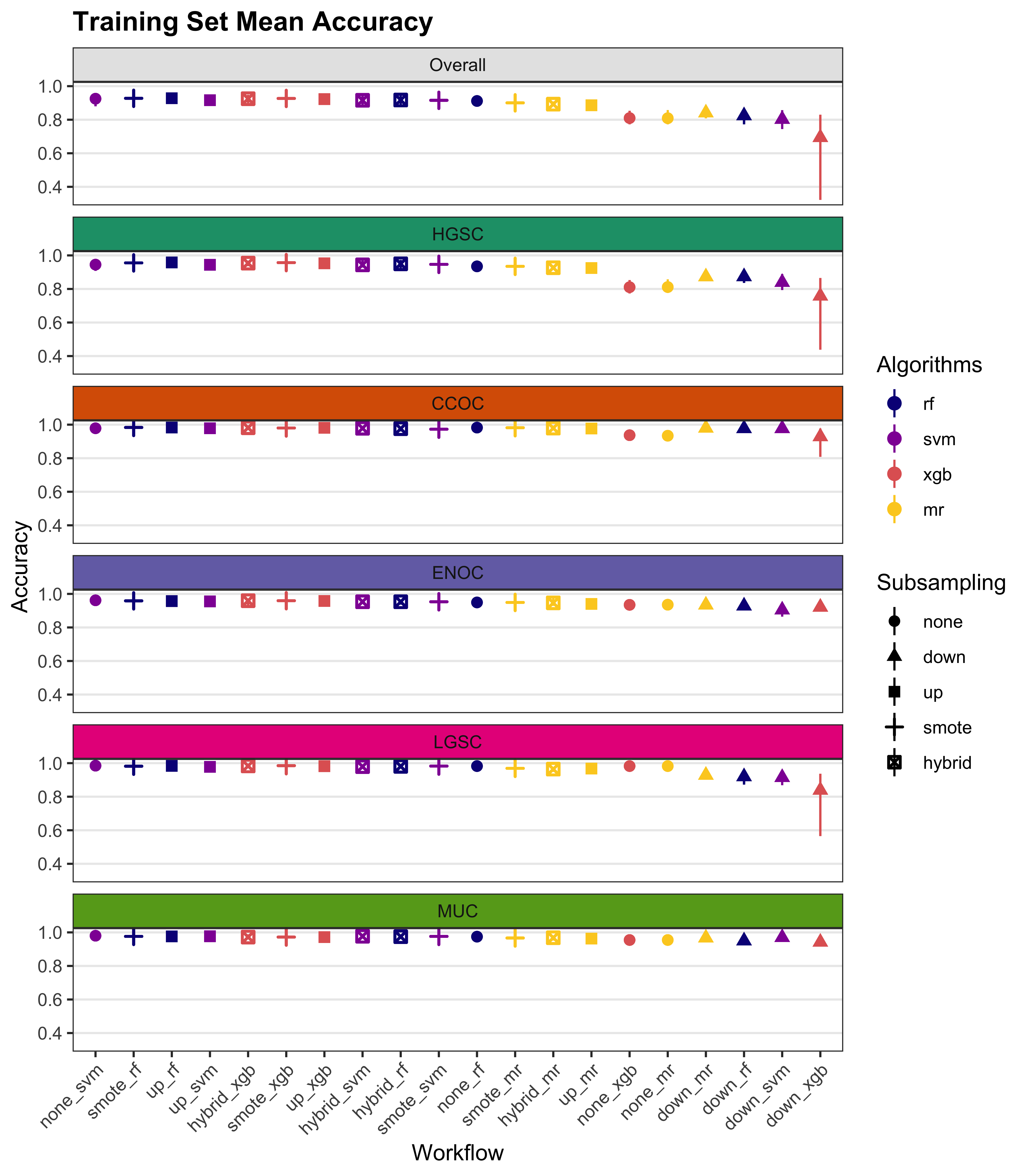
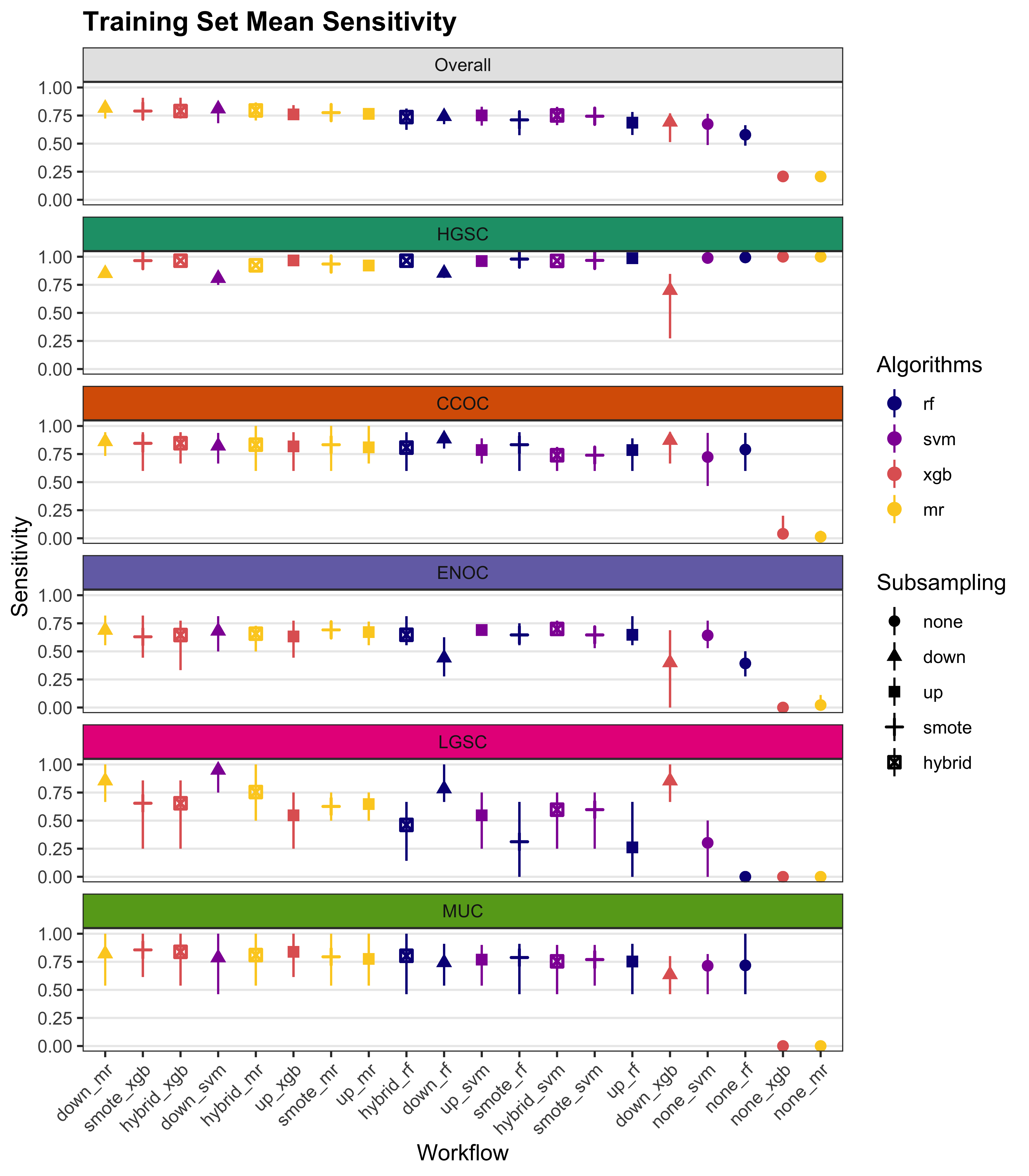
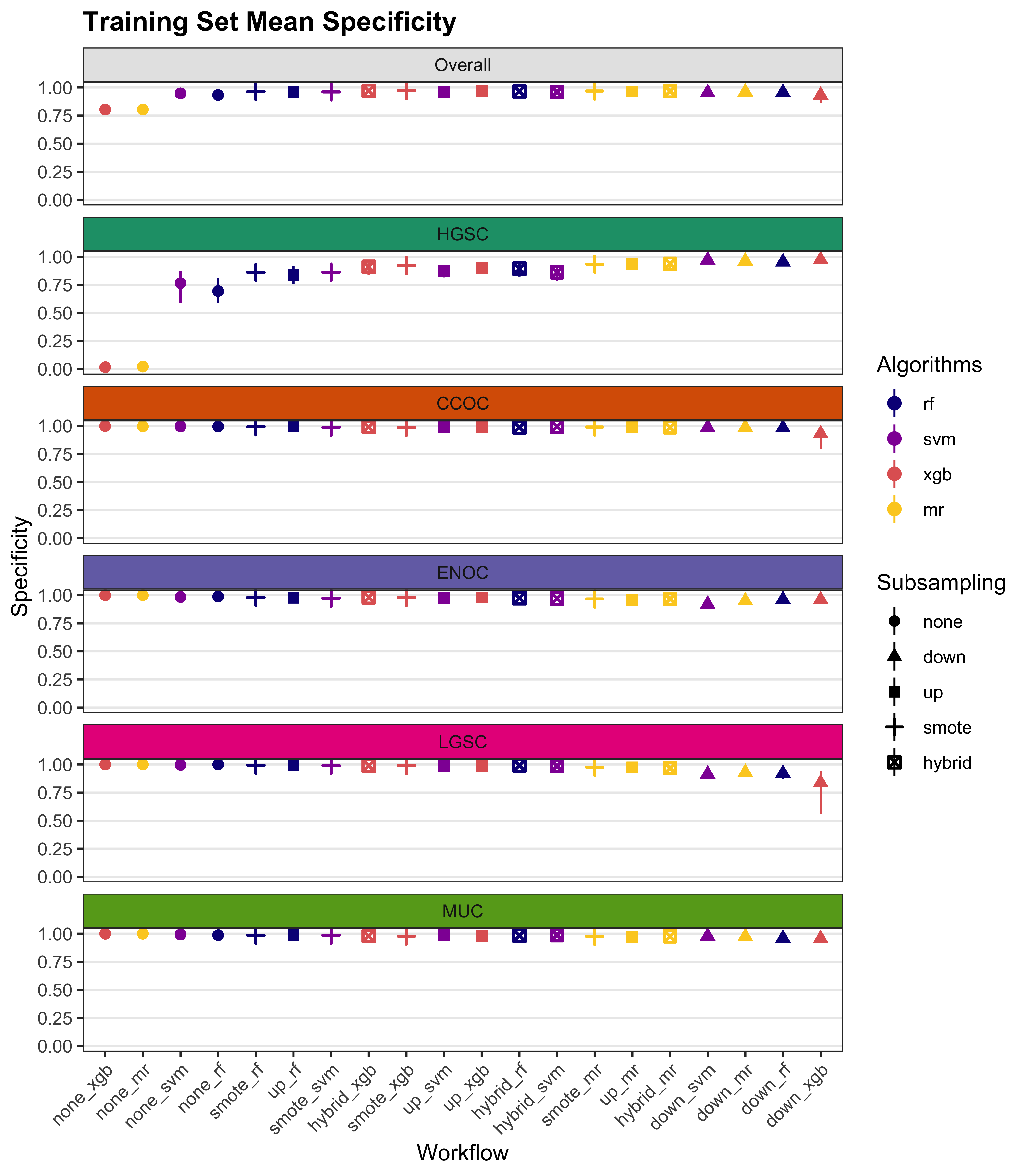
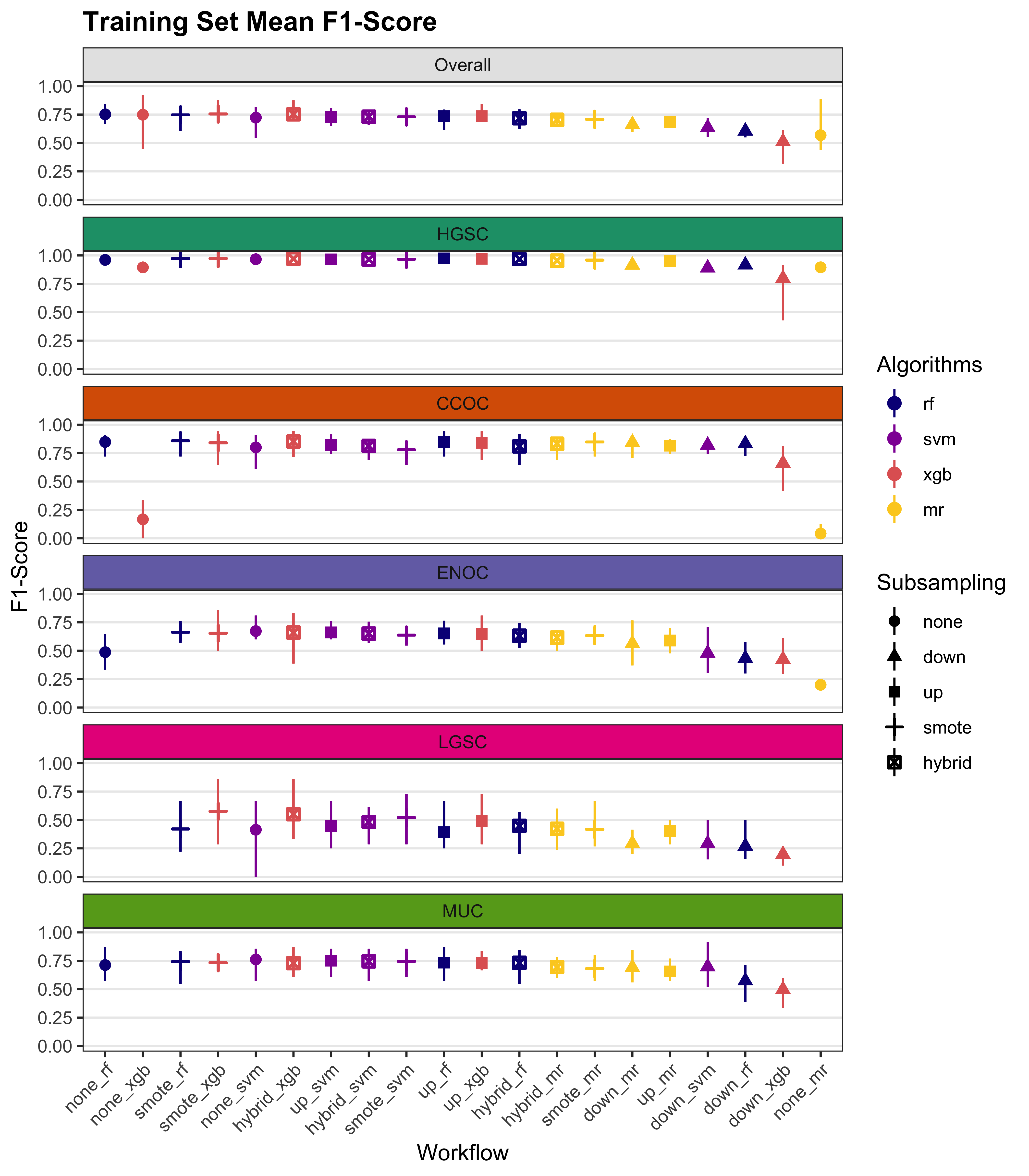
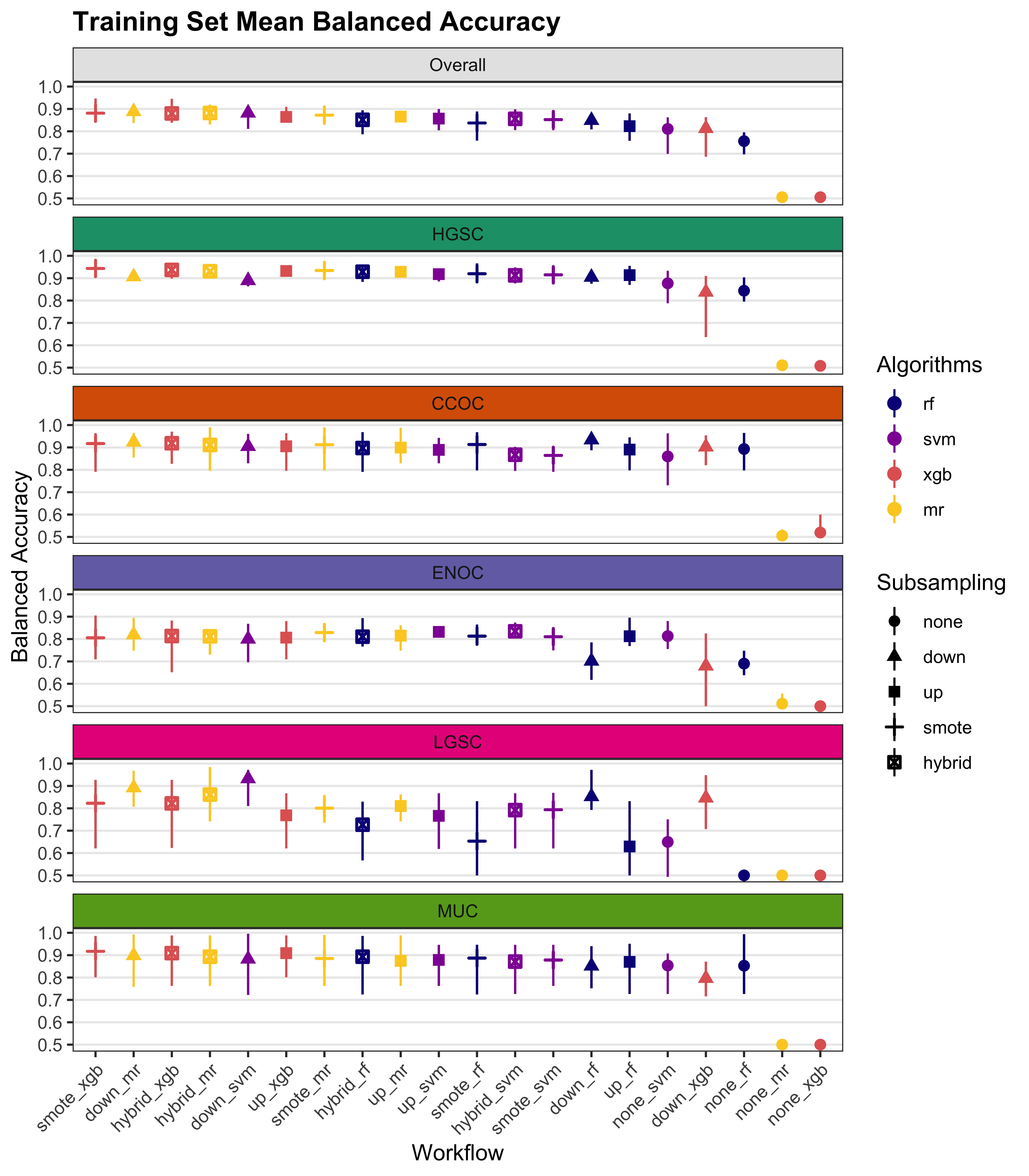
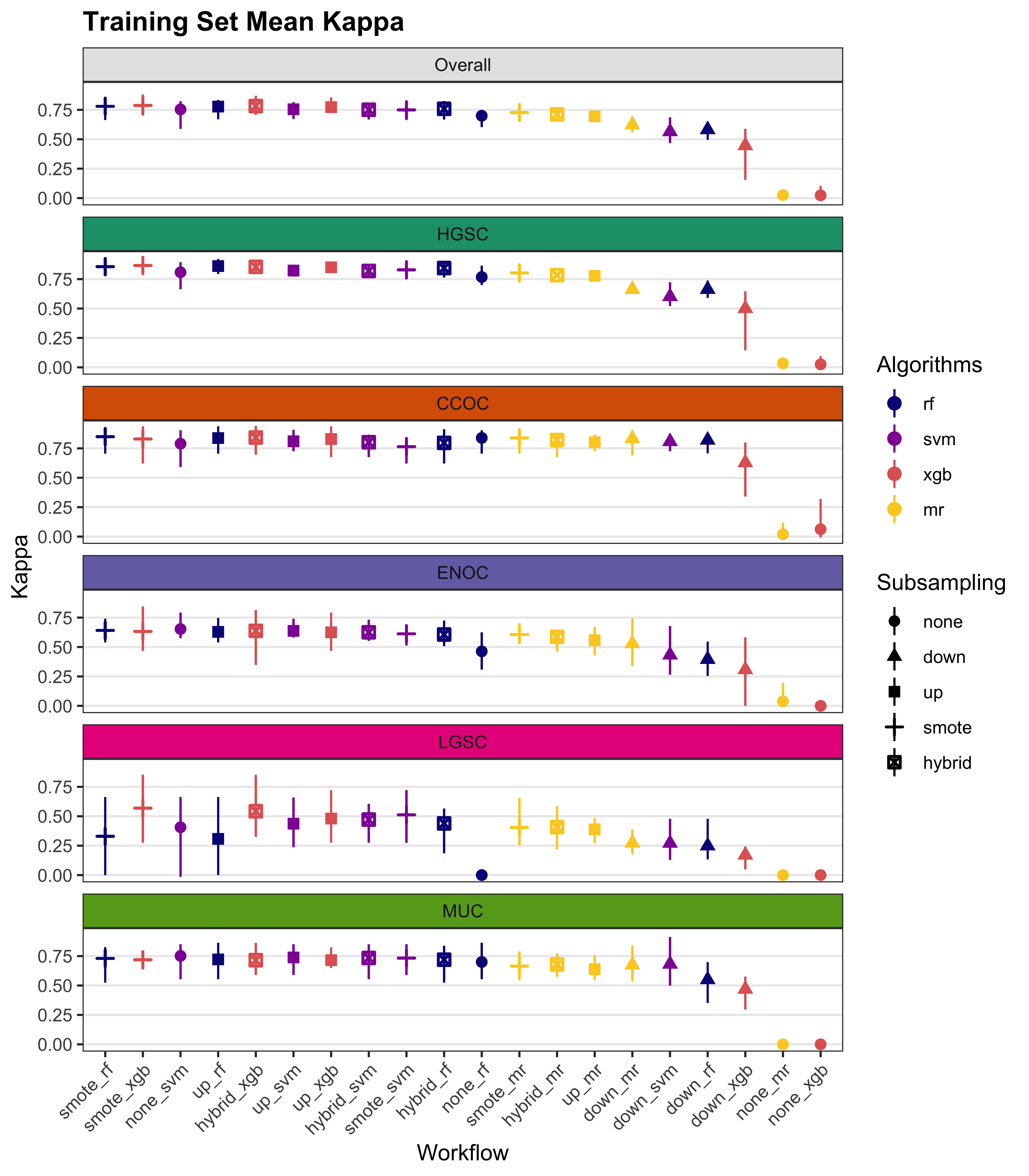
We summarize cross-validated training performance of class metrics in the training set. The accuracy, F1-score, and kappa, are the metrics of interest. Workflows are ordered by their mean estimates across the outer folds of the nested CV for each metric.
4.1 Training Set
| Subsampling | Algorithms | Overall | HGSOC | CCOC | ENOC | MUOC | LGSOC |
|---|---|---|---|---|---|---|---|
| none | rf | 0.636 | 0.994 | 0.794 | 0.498 | 0.728 | 0.167 |
| svm | 0.615 | 0.989 | 0.762 | 0.576 | 0.751 | 0 | |
| xgb | 0.2 | 1 | 0 | 0 | 0 | 0 | |
| mr | 0.2 | 1 | 0 | 0 | 0 | 0 | |
| down | rf | 0.742 | 0.83 | 0.827 | 0.565 | 0.657 | 0.833 |
| svm | 0.779 | 0.805 | 0.759 | 0.611 | 0.836 | 0.883 | |
| xgb | 0.714 | 0.802 | 0.843 | 0.589 | 0.67 | 0.667 | |
| mr | 0.776 | 0.848 | 0.831 | 0.62 | 0.77 | 0.808 | |
| up | rf | 0.673 | 0.988 | 0.793 | 0.635 | 0.766 | 0.183 |
| svm | 0.714 | 0.976 | 0.735 | 0.625 | 0.71 | 0.525 | |
| xgb | 0.718 | 0.981 | 0.805 | 0.624 | 0.781 | 0.4 | |
| mr | 0.788 | 0.921 | 0.849 | 0.666 | 0.786 | 0.717 | |
| smote | rf | 0.658 | 0.984 | 0.748 | 0.618 | 0.75 | 0.192 |
| svm | 0.759 | 0.966 | 0.757 | 0.681 | 0.748 | 0.642 | |
| xgb | 0.777 | 0.965 | 0.831 | 0.615 | 0.804 | 0.667 | |
| mr | 0.788 | 0.93 | 0.835 | 0.654 | 0.802 | 0.717 | |
| hybrid | rf | 0.72 | 0.972 | 0.805 | 0.638 | 0.804 | 0.383 |
| svm | 0.764 | 0.957 | 0.793 | 0.696 | 0.733 | 0.642 | |
| xgb | 0.77 | 0.966 | 0.851 | 0.624 | 0.818 | 0.592 | |
| mr | 0.783 | 0.923 | 0.835 | 0.676 | 0.767 | 0.717 |
| Subsampling | Algorithms | Overall | HGSOC | CCOC | ENOC | MUOC | LGSOC |
|---|---|---|---|---|---|---|---|
| none | rf | 0.946 | 0.764 | 0.996 | 0.985 | 0.988 | 0.999 |
| svm | 0.947 | 0.775 | 0.997 | 0.98 | 0.986 | 1 | |
| xgb | 0.802 | 0.009 | 1 | 0.998 | 1 | 1 | |
| mr | 0.8 | 0 | 1 | 1 | 1 | 1 | |
| down | rf | 0.952 | 0.955 | 0.984 | 0.928 | 0.973 | 0.921 |
| svm | 0.949 | 0.952 | 0.987 | 0.902 | 0.976 | 0.928 | |
| xgb | 0.949 | 0.965 | 0.976 | 0.918 | 0.975 | 0.911 | |
| mr | 0.958 | 0.963 | 0.986 | 0.931 | 0.971 | 0.94 | |
| up | rf | 0.957 | 0.822 | 0.996 | 0.98 | 0.989 | 0.997 |
| svm | 0.958 | 0.844 | 0.99 | 0.973 | 0.992 | 0.993 | |
| xgb | 0.964 | 0.867 | 0.994 | 0.982 | 0.983 | 0.993 | |
| mr | 0.967 | 0.938 | 0.985 | 0.968 | 0.975 | 0.971 | |
| smote | rf | 0.958 | 0.839 | 0.996 | 0.975 | 0.981 | 0.998 |
| svm | 0.964 | 0.88 | 0.993 | 0.971 | 0.989 | 0.987 | |
| xgb | 0.969 | 0.91 | 0.99 | 0.978 | 0.98 | 0.99 | |
| mr | 0.968 | 0.934 | 0.988 | 0.971 | 0.976 | 0.971 | |
| hybrid | rf | 0.964 | 0.874 | 0.992 | 0.974 | 0.984 | 0.994 |
| svm | 0.965 | 0.89 | 0.994 | 0.968 | 0.987 | 0.985 | |
| xgb | 0.969 | 0.904 | 0.992 | 0.98 | 0.979 | 0.989 | |
| mr | 0.967 | 0.934 | 0.987 | 0.965 | 0.977 | 0.97 |
| Subsampling | Algorithms | Overall | HGSOC | CCOC | ENOC | MUOC | LGSOC |
|---|---|---|---|---|---|---|---|
| none | rf | 0.733 | 0.968 | 0.848 | 0.568 | 0.723 | 0.4 |
| svm | 0.782 | 0.968 | 0.834 | 0.607 | 0.719 | NaN | |
| xgb | 0.712 | 0.894 | NaN | 0 | NaN | NaN | |
| mr | 0.893 | 0.893 | NaN | NaN | NaN | NaN | |
| down | rf | 0.594 | 0.901 | 0.799 | 0.419 | 0.589 | 0.262 |
| svm | 0.617 | 0.886 | 0.778 | 0.412 | 0.713 | 0.295 | |
| xgb | 0.576 | 0.886 | 0.771 | 0.42 | 0.608 | 0.194 | |
| mr | 0.628 | 0.913 | 0.817 | 0.47 | 0.638 | 0.302 | |
| up | rf | 0.755 | 0.972 | 0.849 | 0.652 | 0.757 | 0.362 |
| svm | 0.725 | 0.97 | 0.778 | 0.605 | 0.75 | 0.521 | |
| xgb | 0.723 | 0.974 | 0.844 | 0.651 | 0.728 | 0.416 | |
| mr | 0.695 | 0.951 | 0.816 | 0.619 | 0.674 | 0.413 | |
| smote | rf | 0.68 | 0.972 | 0.82 | 0.616 | 0.688 | 0.304 |
| svm | 0.739 | 0.969 | 0.811 | 0.638 | 0.752 | 0.524 | |
| xgb | 0.744 | 0.972 | 0.833 | 0.628 | 0.71 | 0.579 | |
| mr | 0.704 | 0.956 | 0.827 | 0.629 | 0.691 | 0.418 | |
| hybrid | rf | 0.724 | 0.971 | 0.829 | 0.631 | 0.741 | 0.45 |
| svm | 0.733 | 0.965 | 0.838 | 0.635 | 0.72 | 0.507 | |
| xgb | 0.741 | 0.971 | 0.86 | 0.643 | 0.716 | 0.515 | |
| mr | 0.696 | 0.952 | 0.821 | 0.613 | 0.682 | 0.412 |
| Subsampling | Algorithms | Overall | HGSOC | CCOC | ENOC | MUOC | LGSOC |
|---|---|---|---|---|---|---|---|
| none | rf | 0.791 | 0.879 | 0.895 | 0.741 | 0.858 | 0.583 |
| svm | 0.781 | 0.882 | 0.879 | 0.778 | 0.868 | 0.5 | |
| xgb | 0.501 | 0.505 | 0.5 | 0.499 | 0.5 | 0.5 | |
| mr | 0.5 | 0.5 | 0.5 | 0.5 | 0.5 | 0.5 | |
| down | rf | 0.847 | 0.892 | 0.905 | 0.746 | 0.815 | 0.877 |
| svm | 0.864 | 0.879 | 0.873 | 0.757 | 0.906 | 0.906 | |
| xgb | 0.832 | 0.883 | 0.91 | 0.753 | 0.822 | 0.789 | |
| mr | 0.867 | 0.906 | 0.909 | 0.776 | 0.87 | 0.874 | |
| up | rf | 0.815 | 0.905 | 0.894 | 0.808 | 0.878 | 0.59 |
| svm | 0.836 | 0.91 | 0.862 | 0.799 | 0.851 | 0.759 | |
| xgb | 0.841 | 0.924 | 0.9 | 0.803 | 0.882 | 0.696 | |
| mr | 0.878 | 0.93 | 0.917 | 0.817 | 0.881 | 0.844 | |
| smote | rf | 0.808 | 0.911 | 0.872 | 0.797 | 0.865 | 0.595 |
| svm | 0.862 | 0.923 | 0.875 | 0.826 | 0.869 | 0.814 | |
| xgb | 0.873 | 0.938 | 0.911 | 0.797 | 0.892 | 0.828 | |
| mr | 0.878 | 0.932 | 0.912 | 0.813 | 0.889 | 0.844 | |
| hybrid | rf | 0.842 | 0.923 | 0.898 | 0.806 | 0.894 | 0.689 |
| svm | 0.864 | 0.923 | 0.893 | 0.832 | 0.86 | 0.814 | |
| xgb | 0.87 | 0.935 | 0.922 | 0.802 | 0.899 | 0.791 | |
| mr | 0.875 | 0.928 | 0.911 | 0.821 | 0.872 | 0.843 |
| Subsampling | Algorithms | Overall | HGSOC | CCOC | ENOC | MUOC | LGSOC |
|---|---|---|---|---|---|---|---|
| none | rf | 0.744 | 0.822 | 0.84 | 0.545 | 0.711 | 0.237 |
| svm | 0.741 | 0.818 | 0.825 | 0.583 | 0.706 | 0 | |
| xgb | 0.007 | 0.016 | 0 | -0.003 | 0 | 0 | |
| mr | 0 | 0 | 0 | 0 | 0 | 0 | |
| down | rf | 0.55 | 0.621 | 0.785 | 0.37 | 0.568 | 0.24 |
| svm | 0.539 | 0.584 | 0.764 | 0.359 | 0.697 | 0.275 | |
| xgb | 0.519 | 0.584 | 0.754 | 0.37 | 0.588 | 0.17 | |
| mr | 0.595 | 0.657 | 0.805 | 0.426 | 0.618 | 0.282 | |
| up | rf | 0.776 | 0.85 | 0.84 | 0.63 | 0.746 | 0.213 |
| svm | 0.749 | 0.835 | 0.764 | 0.579 | 0.739 | 0.513 | |
| xgb | 0.781 | 0.865 | 0.835 | 0.63 | 0.714 | 0.408 | |
| mr | 0.708 | 0.778 | 0.803 | 0.592 | 0.657 | 0.399 | |
| smote | rf | 0.756 | 0.853 | 0.81 | 0.591 | 0.673 | 0.299 |
| svm | 0.761 | 0.839 | 0.8 | 0.614 | 0.741 | 0.516 | |
| xgb | 0.773 | 0.856 | 0.822 | 0.604 | 0.695 | 0.571 | |
| mr | 0.72 | 0.793 | 0.816 | 0.603 | 0.675 | 0.405 | |
| hybrid | rf | 0.767 | 0.85 | 0.818 | 0.605 | 0.728 | 0.443 |
| svm | 0.753 | 0.825 | 0.828 | 0.609 | 0.707 | 0.497 | |
| xgb | 0.778 | 0.855 | 0.852 | 0.62 | 0.702 | 0.506 | |
| mr | 0.707 | 0.779 | 0.81 | 0.585 | 0.665 | 0.399 |
4.2 Rank Aggregation
Multi-step methods:
- sequential: sequential algorithm sequence of subsampling methods and algorithms used are:
- HGSOC vs. non-HGSOC using upsampling and XGBoost
- CCOC vs. non-CCOC using SMOTE subsampling and XGBoost
- ENOC vs. non-ENOC using no subsampling and support vector machine
- MUOC vs. LGSOC using SMOTE subsampling and random forest
- two_step: two-step algorithm sequence of subsampling methods and algorithms used are:
- HGSOC vs. non-HGSOC using upsampling and XGBoost
- CCOC vs. ENOC vs. MUOC vs. LGSOC using SMOTE subsampling and support vector machine
We conduct rank aggregation using a two-stage nested approach:
- First we rank aggregate the per-class metrics for F1-score, balanced accuracy and kappa.
- Then we take the aggregated lists from the three metrics and perform a final rank aggregation.
- The top workflows from the final rank aggregation are used for gene optimization in the confirmation set
4.2.1 Across Classes
4.2.2 Across Metrics
| Rank | F1 | Balanced Accuracy | Kappa |
|---|---|---|---|
| 1 | sequential | sequential | sequential |
| 2 | two_step | hybrid_xgb | two_step |
| 3 | up_rf | up_mr | smote_svm |
| 4 | smote_svm | smote_mr | up_rf |
| 5 | hybrid_xgb | smote_xgb | up_xgb |
| 6 | up_xgb | two_step | hybrid_xgb |
| 7 | hybrid_svm | hybrid_mr | hybrid_svm |
| 8 | hybrid_rf | up_xgb | hybrid_rf |
| 9 | smote_xgb | hybrid_svm | smote_xgb |
| 10 | smote_mr | smote_svm | up_svm |
| 11 | up_svm | down_mr | smote_mr |
| 12 | smote_rf | hybrid_rf | smote_rf |
| 13 | none_rf | up_svm | none_svm |
| 14 | hybrid_mr | up_rf | none_rf |
| 15 | up_mr | smote_rf | hybrid_mr |
| 16 | down_mr | down_rf | up_mr |
| 17 | down_svm | down_xgb | down_mr |
| 18 | down_rf | none_svm | down_rf |
| 19 | down_xgb | none_rf | down_xgb |
| 20 | NA | down_svm | down_svm |
| 21 | NA | none_mr | none_mr |
| 22 | NA | none_xgb | none_xgb |
| Rank | Workflow |
|---|---|
| 1 | sequential |
| 2 | two_step |
| 3 | up_rf |
| 4 | smote_svm |
| 5 | hybrid_xgb |
4.2.3 Top Workflows
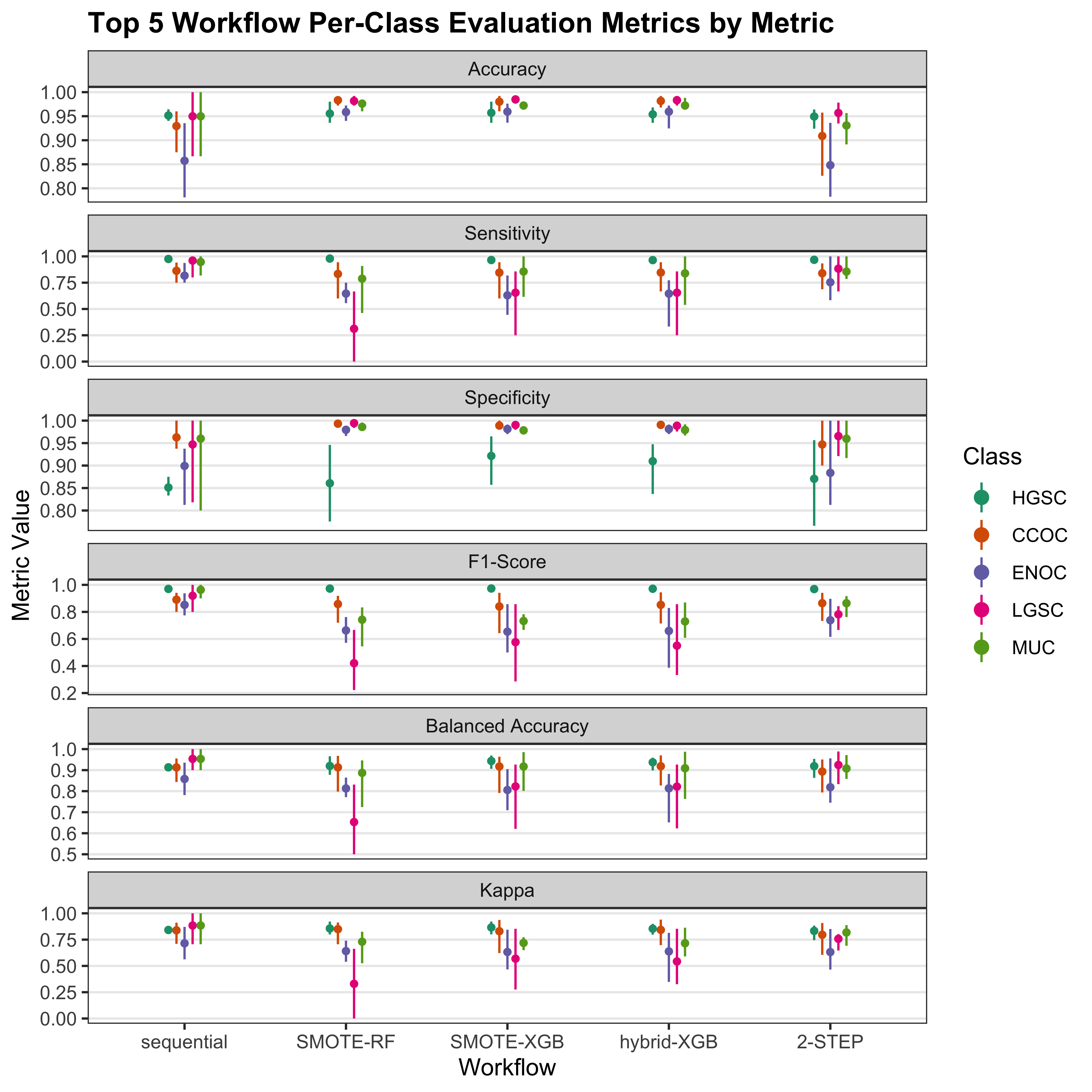
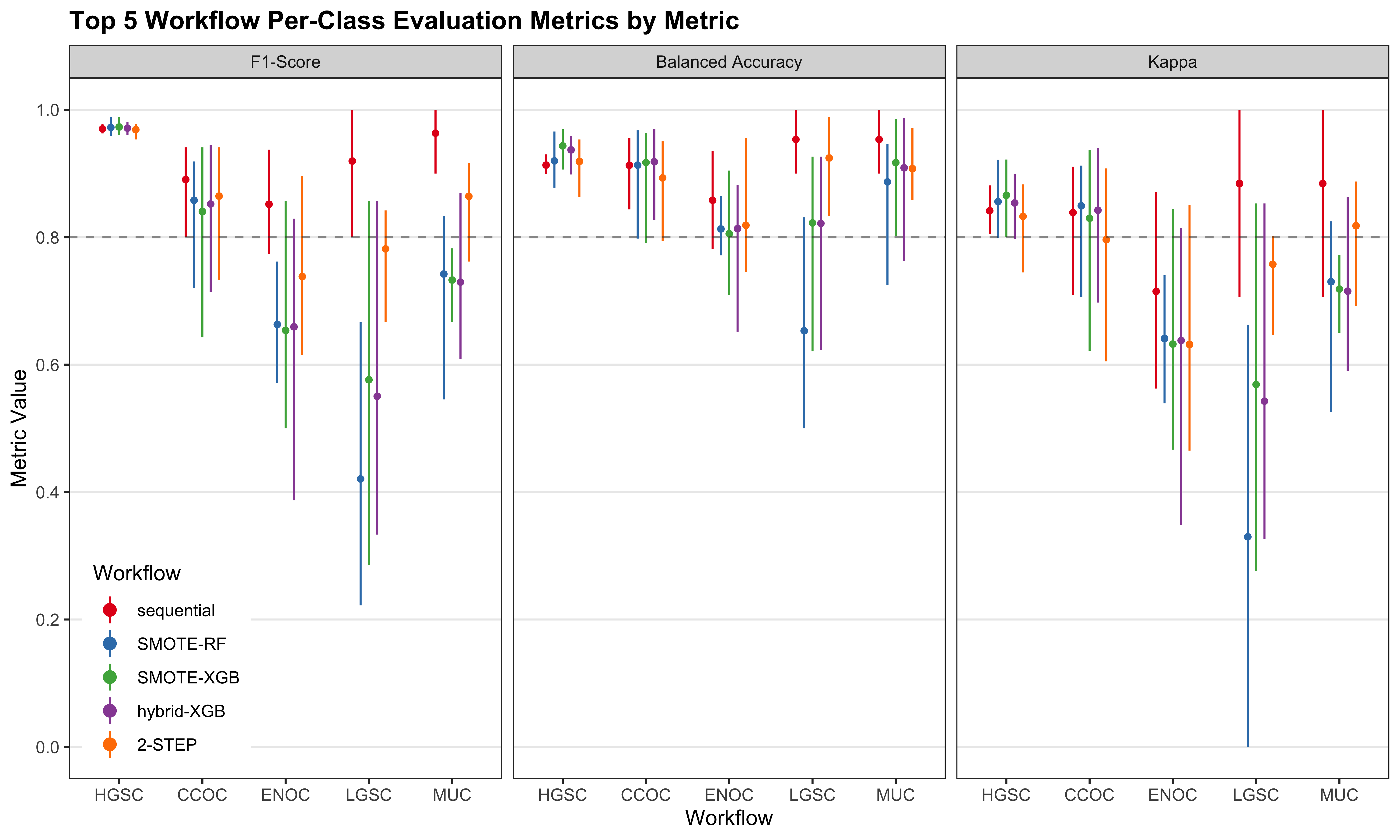
We look at the per-class evaluation metrics of the top 5 workflows.
| Metric | Workflow | HGSOC | CCOC | ENOC | MUOC | LGSOC |
|---|---|---|---|---|---|---|
| Accuracy | Sequential | 0.96 (0.95, 0.96) | 0.92 (0.88, 0.96) | 0.86 (0.77, 0.91) | 0.95 (0.88, 1) | 0.95 (0.88, 1) |
| 2-STEP | 0.96 (0.95, 0.96) | 0.93 (0.9, 0.96) | 0.84 (0.73, 0.9) | 0.89 (0.81, 0.96) | 0.97 (0.94, 1) | |
| Up-RF | 0.95 (0.92, 0.98) | 0.98 (0.97, 0.99) | 0.96 (0.95, 0.97) | 0.98 (0.96, 0.99) | 0.98 (0.97, 0.99) | |
| SMOTE-SVM | 0.95 (0.94, 0.97) | 0.98 (0.97, 0.99) | 0.95 (0.94, 0.96) | 0.98 (0.96, 0.98) | 0.98 (0.97, 0.98) | |
| Hybrid-XGB | 0.95 (0.94, 0.97) | 0.98 (0.97, 0.99) | 0.96 (0.94, 0.97) | 0.97 (0.96, 0.98) | 0.98 (0.97, 0.99) | |
| Sensitivity | Sequential | 0.98 (0.97, 0.99) | 0.88 (0.81, 1) | 0.86 (0.81, 0.94) | 0.97 (0.91, 1) | 0.92 (0.6, 1) |
| 2-STEP | 0.98 (0.97, 0.99) | 0.87 (0.82, 0.93) | 0.73 (0.56, 0.82) | 0.84 (0.75, 0.92) | 0.77 (0, 1) | |
| Up-RF | 0.99 (0.98, 1) | 0.79 (0.57, 0.88) | 0.64 (0.44, 0.81) | 0.77 (0.46, 0.91) | 0.18 (0, 0.33) | |
| SMOTE-SVM | 0.97 (0.96, 0.98) | 0.76 (0.57, 0.85) | 0.68 (0.5, 0.86) | 0.75 (0.54, 0.91) | 0.64 (0.5, 0.75) | |
| Hybrid-XGB | 0.97 (0.96, 0.98) | 0.85 (0.57, 0.95) | 0.62 (0.44, 0.77) | 0.82 (0.54, 0.91) | 0.59 (0.38, 0.75) | |
| Specificity | Sequential | 0.88 (0.85, 0.9) | 0.94 (0.85, 1) | 0.85 (0.73, 0.88) | 0.92 (0.6, 1) | 0.97 (0.91, 1) |
| 2-STEP | 0.88 (0.85, 0.9) | 0.97 (0.94, 1) | 0.89 (0.83, 0.94) | 0.91 (0.83, 0.97) | 0.98 (0.95, 1) | |
| Up-RF | 0.82 (0.74, 0.89) | 1 (0.99, 1) | 0.98 (0.97, 0.99) | 0.99 (0.98, 1) | 1 (0.99, 1) | |
| SMOTE-SVM | 0.88 (0.8, 0.92) | 0.99 (0.99, 1) | 0.97 (0.96, 0.98) | 0.99 (0.98, 1) | 0.99 (0.98, 1) | |
| Hybrid-XGB | 0.9 (0.85, 0.95) | 0.99 (0.99, 1) | 0.98 (0.97, 0.99) | 0.98 (0.97, 0.99) | 0.99 (0.98, 0.99) | |
| F1-Score | Sequential | 0.97 (0.97, 0.98) | 0.88 (0.81, 0.94) | 0.86 (0.79, 0.91) | 0.97 (0.92, 1) | 0.91 (0.75, 1) |
| 2-STEP | 0.97 (0.97, 0.98) | 0.9 (0.85, 0.93) | 0.75 (0.61, 0.85) | 0.79 (0.67, 0.92) | 0.73 (0, 1) | |
| Up-RF | 0.97 (0.95, 0.99) | 0.85 (0.7, 0.94) | 0.65 (0.47, 0.79) | 0.76 (0.57, 0.87) | 0.36 (0.29, 0.4) | |
| SMOTE-SVM | 0.97 (0.96, 0.98) | 0.81 (0.67, 0.92) | 0.64 (0.5, 0.81) | 0.75 (0.58, 0.83) | 0.52 (0.36, 0.71) | |
| Hybrid-XGB | 0.97 (0.96, 0.98) | 0.86 (0.67, 0.95) | 0.64 (0.5, 0.81) | 0.72 (0.61, 0.8) | 0.51 (0.44, 0.67) | |
| Balanced Accuracy | Sequential | 0.93 (0.91, 0.94) | 0.91 (0.86, 0.95) | 0.86 (0.77, 0.91) | 0.94 (0.8, 1) | 0.94 (0.8, 1) |
| 2-STEP | 0.93 (0.91, 0.94) | 0.92 (0.88, 0.95) | 0.81 (0.69, 0.88) | 0.87 (0.79, 0.95) | 0.87 (0.48, 1) | |
| Up-RF | 0.9 (0.86, 0.94) | 0.89 (0.78, 0.94) | 0.81 (0.71, 0.9) | 0.88 (0.73, 0.95) | 0.59 (0.5, 0.66) | |
| SMOTE-SVM | 0.92 (0.89, 0.95) | 0.88 (0.78, 0.92) | 0.83 (0.74, 0.92) | 0.87 (0.76, 0.95) | 0.81 (0.75, 0.87) | |
| Hybrid-XGB | 0.94 (0.91, 0.96) | 0.92 (0.78, 0.97) | 0.8 (0.72, 0.88) | 0.9 (0.76, 0.95) | 0.79 (0.68, 0.87) | |
| Kappa | Sequential | 0.86 (0.83, 0.88) | 0.82 (0.72, 0.91) | 0.71 (0.55, 0.82) | 0.88 (0.68, 1) | 0.88 (0.68, 1) |
| 2-STEP | 0.86 (0.83, 0.88) | 0.85 (0.77, 0.9) | 0.63 (0.4, 0.77) | 0.72 (0.54, 0.9) | 0.72 (-0.03, 1) | |
| Up-RF | 0.85 (0.77, 0.9) | 0.84 (0.68, 0.93) | 0.63 (0.45, 0.77) | 0.75 (0.55, 0.86) | 0.21 (0, 0.4) | |
| SMOTE-SVM | 0.84 (0.78, 0.88) | 0.8 (0.65, 0.91) | 0.61 (0.48, 0.79) | 0.74 (0.56, 0.83) | 0.52 (0.35, 0.71) | |
| Hybrid-XGB | 0.85 (0.83, 0.89) | 0.85 (0.65, 0.95) | 0.62 (0.48, 0.79) | 0.7 (0.59, 0.79) | 0.51 (0.44, 0.66) |
| Workflow | Rank | HGSOC | CCOC | ENOC | MUOC | LGSOC |
|---|---|---|---|---|---|---|
| F1-Score | ||||||
| Sequential | 1 | 0.973 | 0.877 | 0.860 | 0.966 | 0.910 |
| 2-STEP | 2 | 0.973 | 0.899 | 0.755 | 0.788 | 0.733 |
| Up-RF | 3 | 0.972 | 0.849 | 0.652 | 0.757 | 0.362 |
| SMOTE-SVM | 4 | 0.969 | 0.811 | 0.638 | 0.752 | 0.524 |
| Hybrid-XGB | 5 | 0.971 | 0.860 | 0.643 | 0.716 | 0.515 |
| Balanced Accuracy | ||||||
| Sequential | 1 | 0.926 | 0.907 | 0.856 | 0.943 | 0.943 |
| Hybrid-XGB | 2 | 0.935 | 0.922 | 0.802 | 0.899 | 0.791 |
| 2-STEP | 6 | 0.926 | 0.917 | 0.814 | 0.875 | 0.872 |
| SMOTE-SVM | 10 | 0.923 | 0.875 | 0.826 | 0.869 | 0.814 |
| Up-RF | 14 | 0.905 | 0.894 | 0.808 | 0.878 | 0.590 |
| Kappa | ||||||
| Sequential | 1 | 0.858 | 0.815 | 0.712 | 0.877 | 0.877 |
| 2-STEP | 2 | 0.858 | 0.850 | 0.635 | 0.716 | 0.718 |
| SMOTE-SVM | 3 | 0.839 | 0.800 | 0.614 | 0.741 | 0.516 |
| Up-RF | 4 | 0.850 | 0.840 | 0.630 | 0.746 | 0.213 |
| Hybrid-XGB | 6 | 0.855 | 0.852 | 0.620 | 0.702 | 0.506 |
Misclassified cases from a previous step of the sequence of classifiers are not included in subsequent steps of the training set CV folds. Thus, we cannot piece together the test set predictions from the sequential and two-step algorithms to obtain overall metrics.
4.3 Confirmation Set
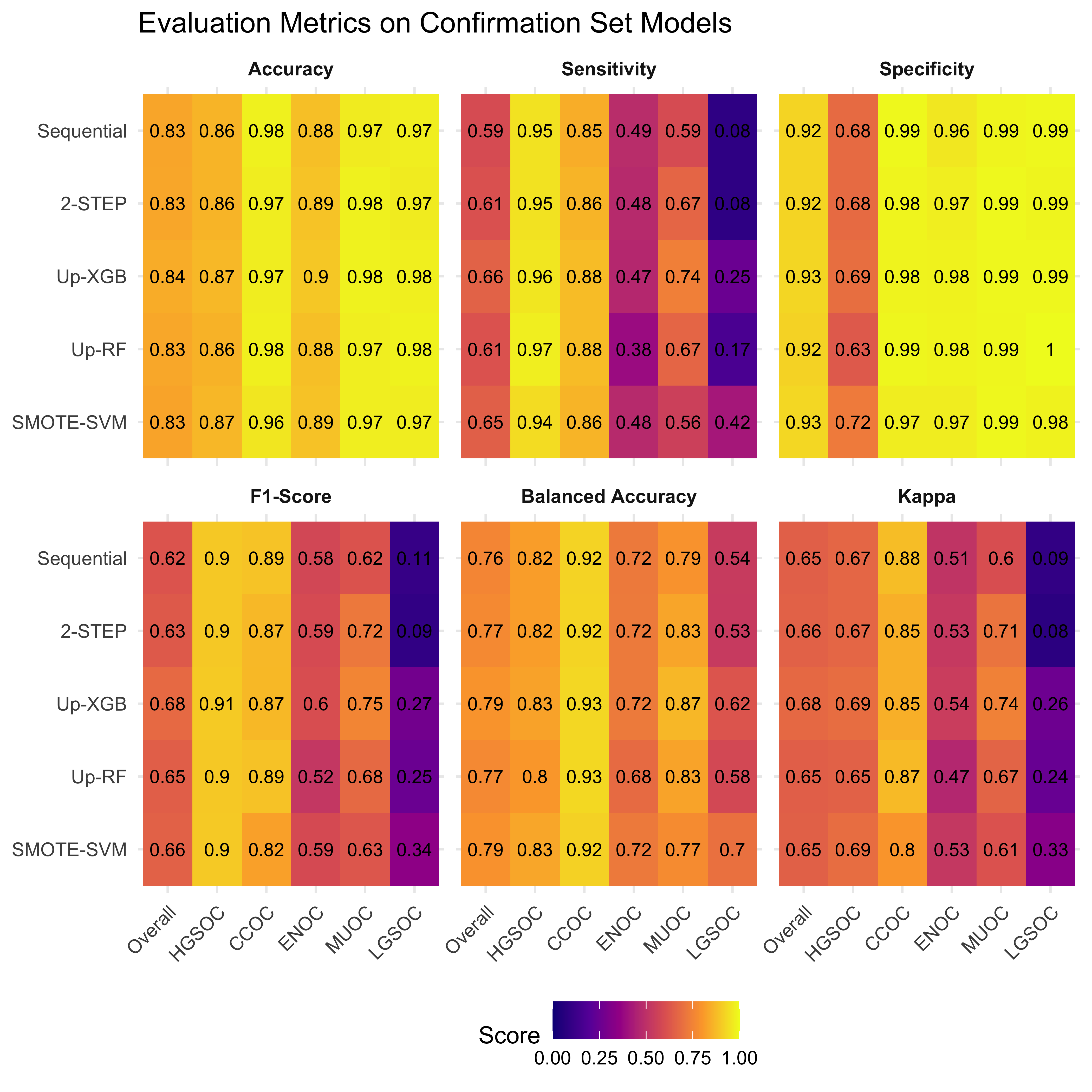
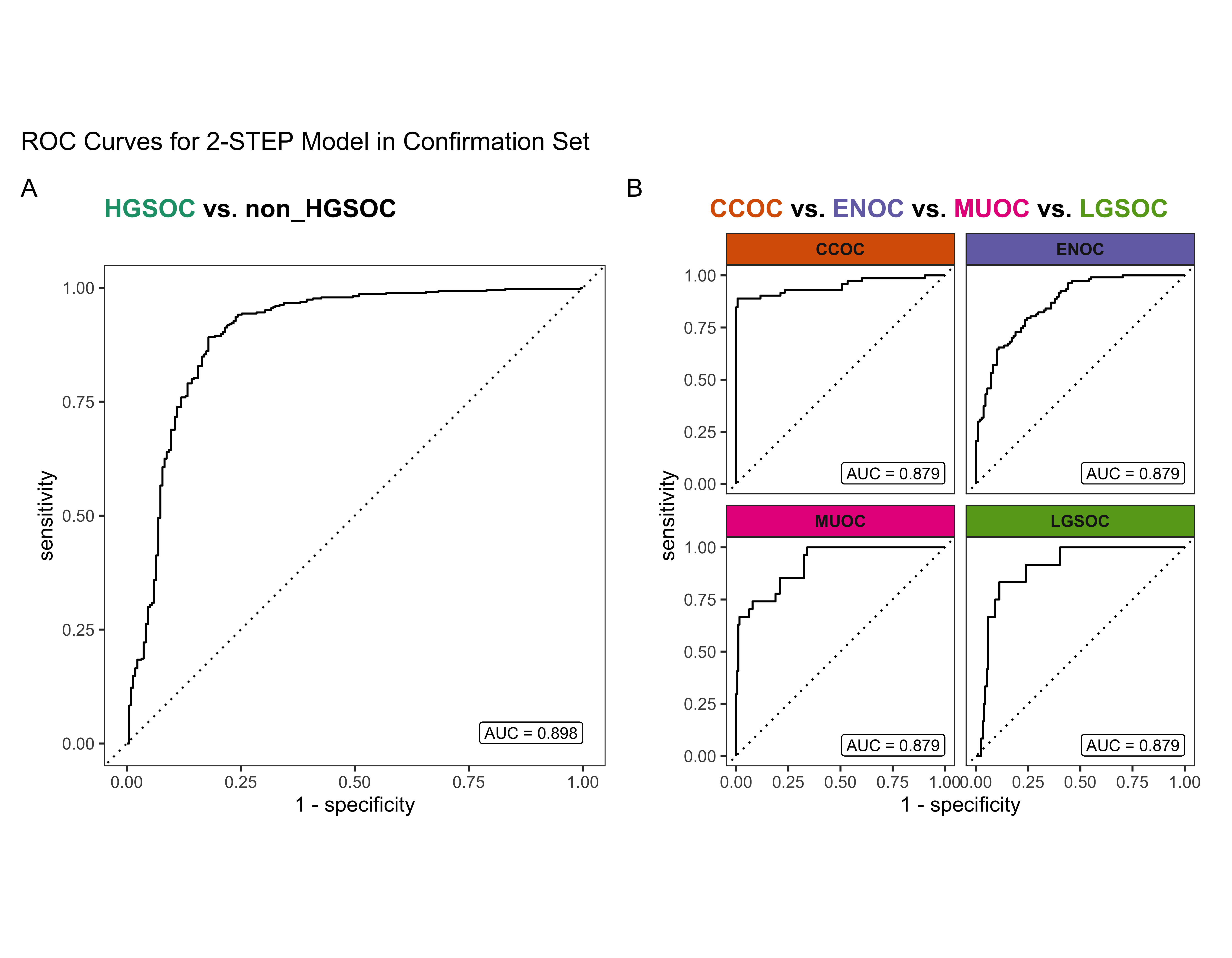
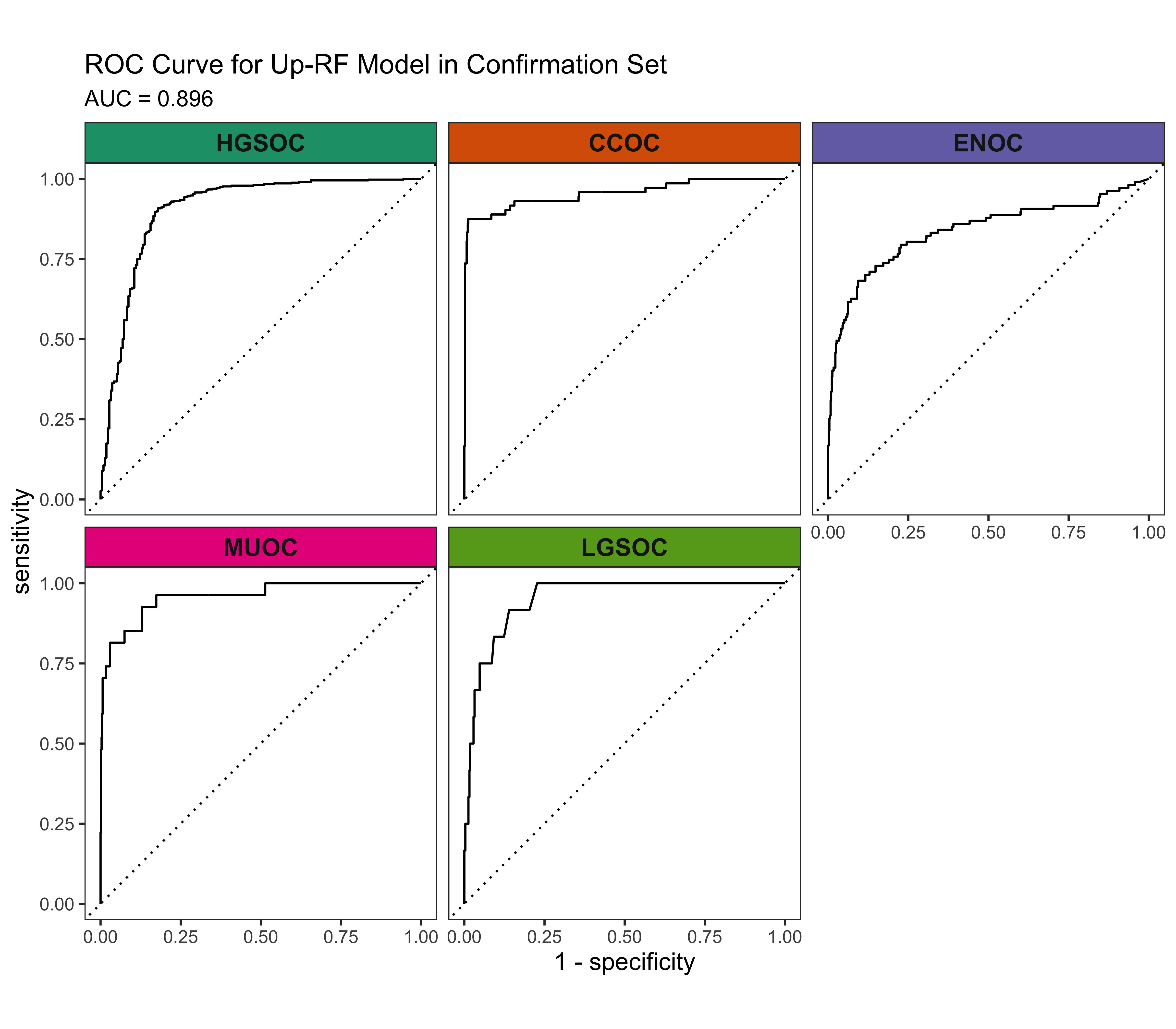
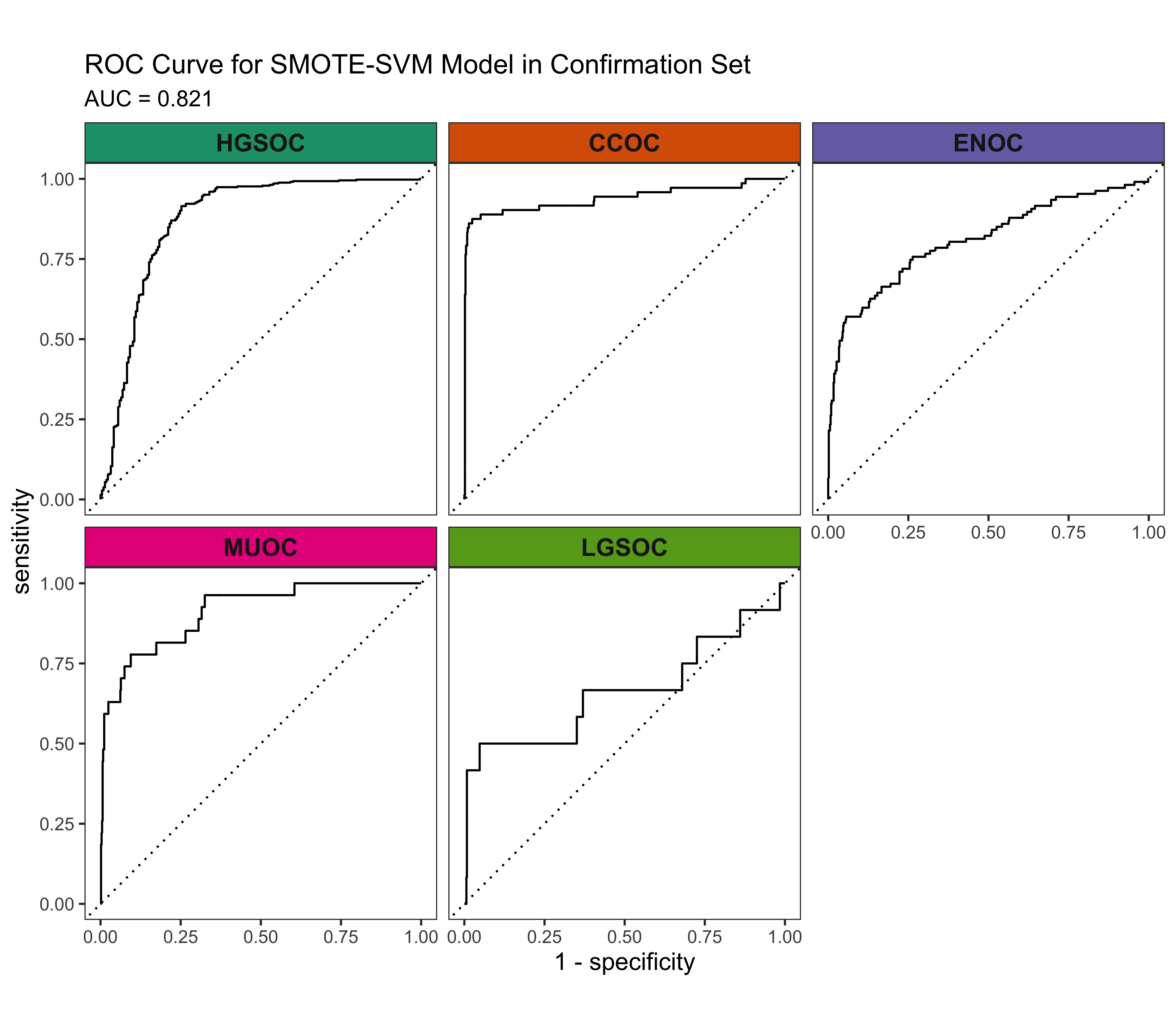
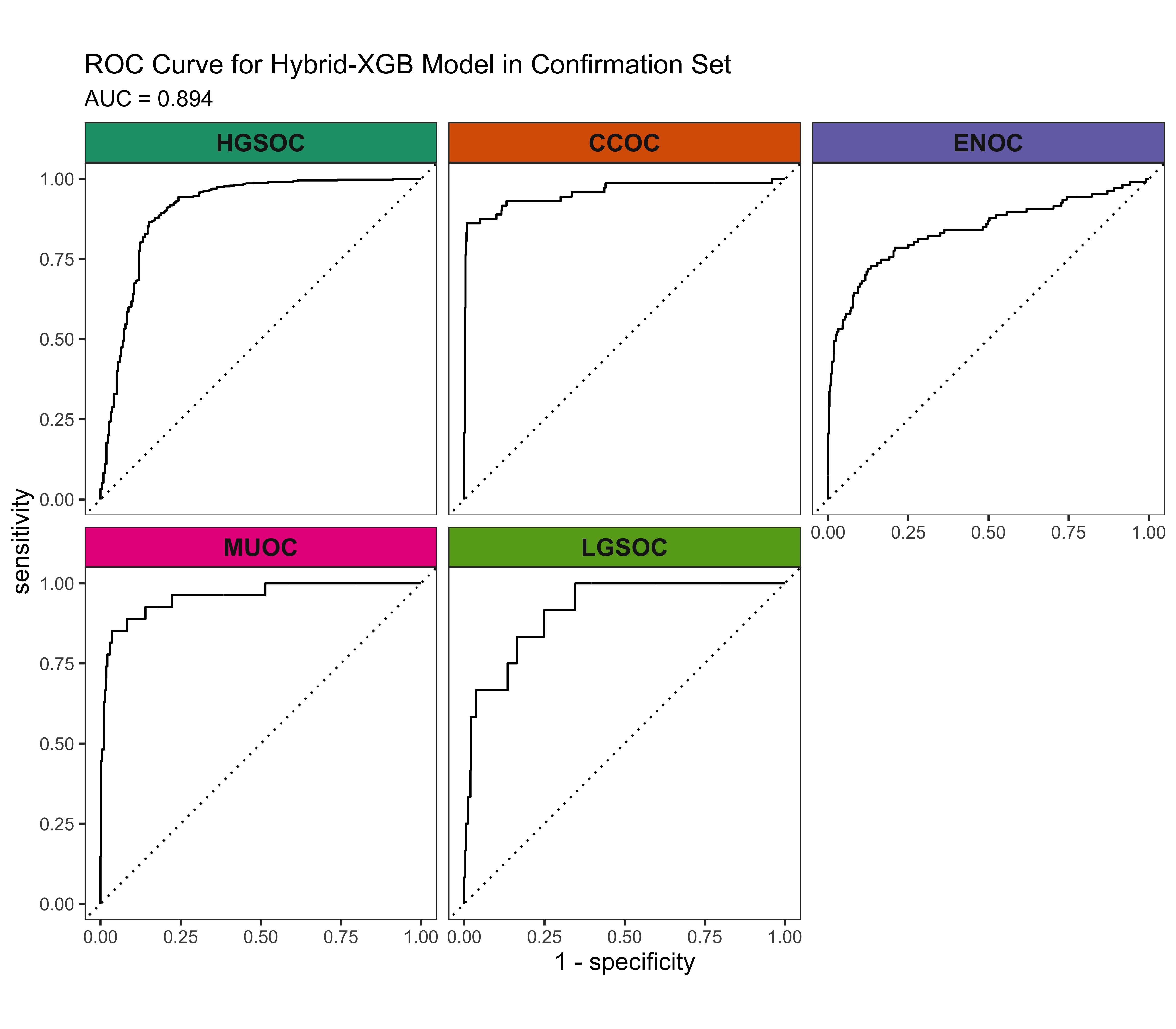
Now we’d like to see how our best five workflows perform in the confirmation set. The class-specific F1-scores will be used. The top performing method will be selected for gene optimization.
| Method | Metric | Overall | HGSOC | CCOC | ENOC | MUOC | LGSOC |
|---|---|---|---|---|---|---|---|
| Sequential | Accuracy | 0.829 | 0.866 | 0.969 | 0.883 | 0.966 | 0.974 |
| Sensitivity | 0.584 | 0.953 | 0.861 | 0.467 | 0.556 | 0.083 | |
| Specificity | 0.924 | 0.697 | 0.982 | 0.966 | 0.984 | 0.990 | |
| F1-Score | 0.604 | 0.904 | 0.861 | 0.571 | 0.577 | 0.105 | |
| Balanced Accuracy | 0.754 | 0.825 | 0.922 | 0.717 | 0.770 | 0.537 | |
| Kappa | 0.646 | 0.685 | 0.844 | 0.508 | 0.559 | 0.093 | |
| 2-STEP | Accuracy | 0.838 | 0.866 | 0.970 | 0.891 | 0.977 | 0.972 |
| Sensitivity | 0.613 | 0.953 | 0.875 | 0.486 | 0.667 | 0.083 | |
| Specificity | 0.926 | 0.697 | 0.982 | 0.972 | 0.990 | 0.989 | |
| F1-Score | 0.635 | 0.904 | 0.869 | 0.598 | 0.706 | 0.100 | |
| Balanced Accuracy | 0.769 | 0.825 | 0.929 | 0.729 | 0.828 | 0.536 | |
| Kappa | 0.666 | 0.685 | 0.852 | 0.538 | 0.694 | 0.086 | |
| Up-RF | Accuracy | 0.835 | 0.857 | 0.975 | 0.883 | 0.974 | 0.981 |
| Sensitivity | 0.613 | 0.972 | 0.875 | 0.383 | 0.667 | 0.167 | |
| Specificity | 0.918 | 0.633 | 0.988 | 0.983 | 0.987 | 0.997 | |
| F1-Score | 0.648 | 0.900 | 0.887 | 0.522 | 0.679 | 0.250 | |
| Balanced Accuracy | 0.765 | 0.802 | 0.931 | 0.683 | 0.827 | 0.582 | |
| Kappa | 0.646 | 0.654 | 0.873 | 0.466 | 0.665 | 0.243 | |
| SMOTE-SVM | Accuracy | 0.827 | 0.866 | 0.958 | 0.888 | 0.972 | 0.970 |
| Sensitivity | 0.650 | 0.939 | 0.861 | 0.477 | 0.556 | 0.417 | |
| Specificity | 0.927 | 0.725 | 0.970 | 0.970 | 0.990 | 0.981 | |
| F1-Score | 0.656 | 0.902 | 0.821 | 0.586 | 0.625 | 0.345 | |
| Balanced Accuracy | 0.788 | 0.832 | 0.916 | 0.723 | 0.773 | 0.699 | |
| Kappa | 0.651 | 0.690 | 0.797 | 0.525 | 0.611 | 0.330 | |
| Hybrid-XGB | Accuracy | 0.830 | 0.869 | 0.961 | 0.893 | 0.967 | 0.970 |
| Sensitivity | 0.662 | 0.943 | 0.861 | 0.458 | 0.630 | 0.417 | |
| Specificity | 0.928 | 0.725 | 0.974 | 0.979 | 0.982 | 0.981 | |
| F1-Score | 0.657 | 0.905 | 0.832 | 0.587 | 0.618 | 0.345 | |
| Balanced Accuracy | 0.795 | 0.834 | 0.917 | 0.719 | 0.806 | 0.699 | |
| Kappa | 0.657 | 0.696 | 0.810 | 0.531 | 0.601 | 0.330 |
4.4 Gene Optimization
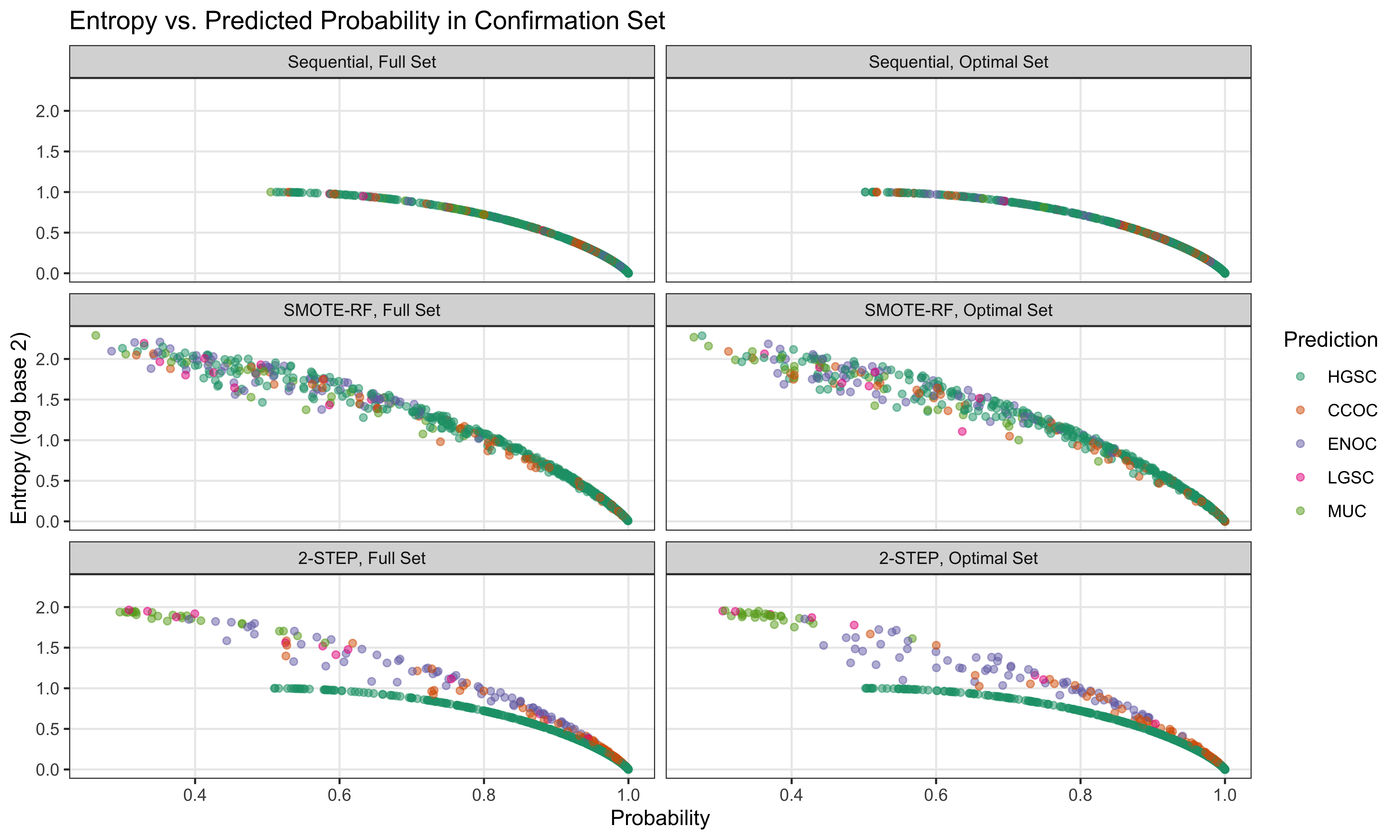
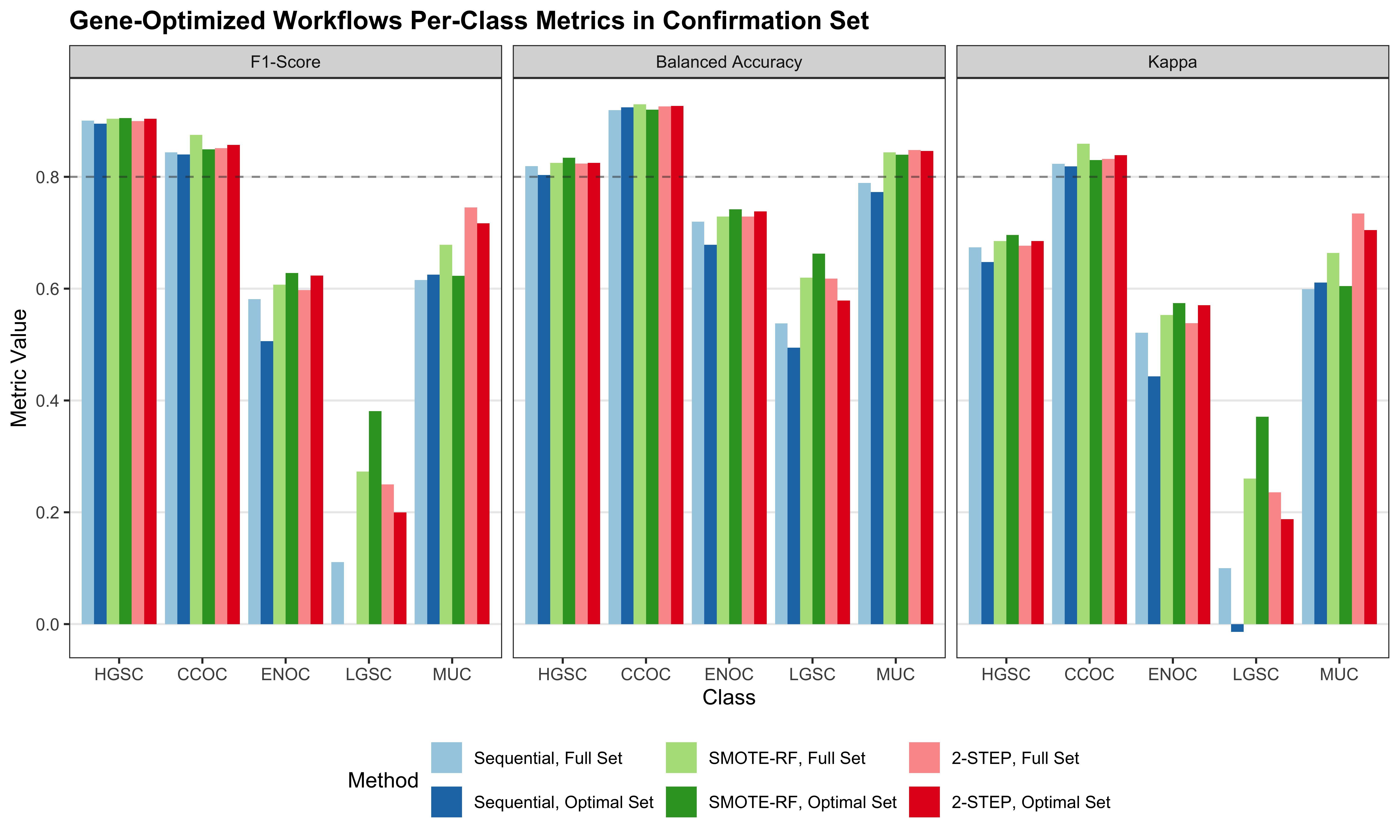
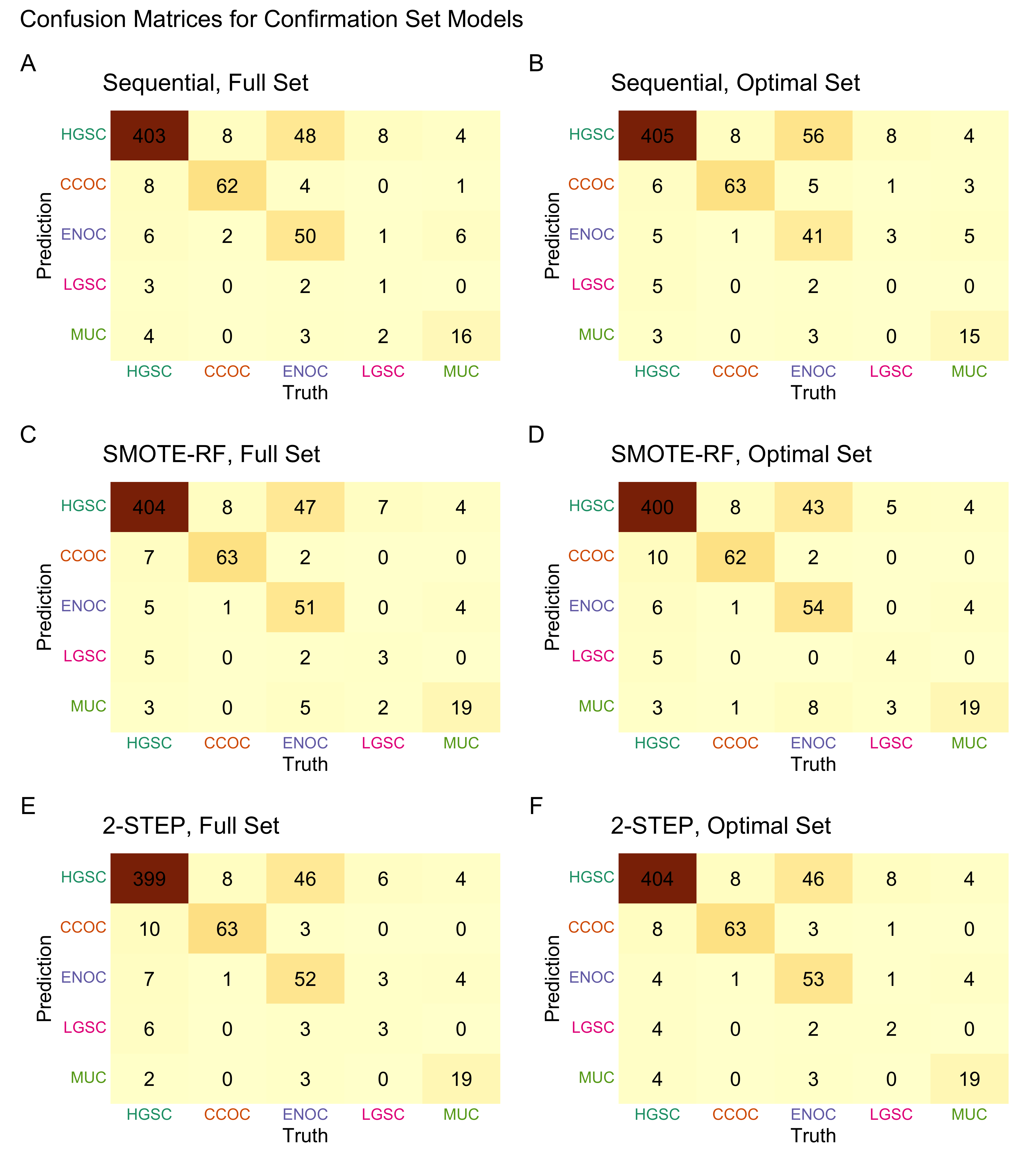
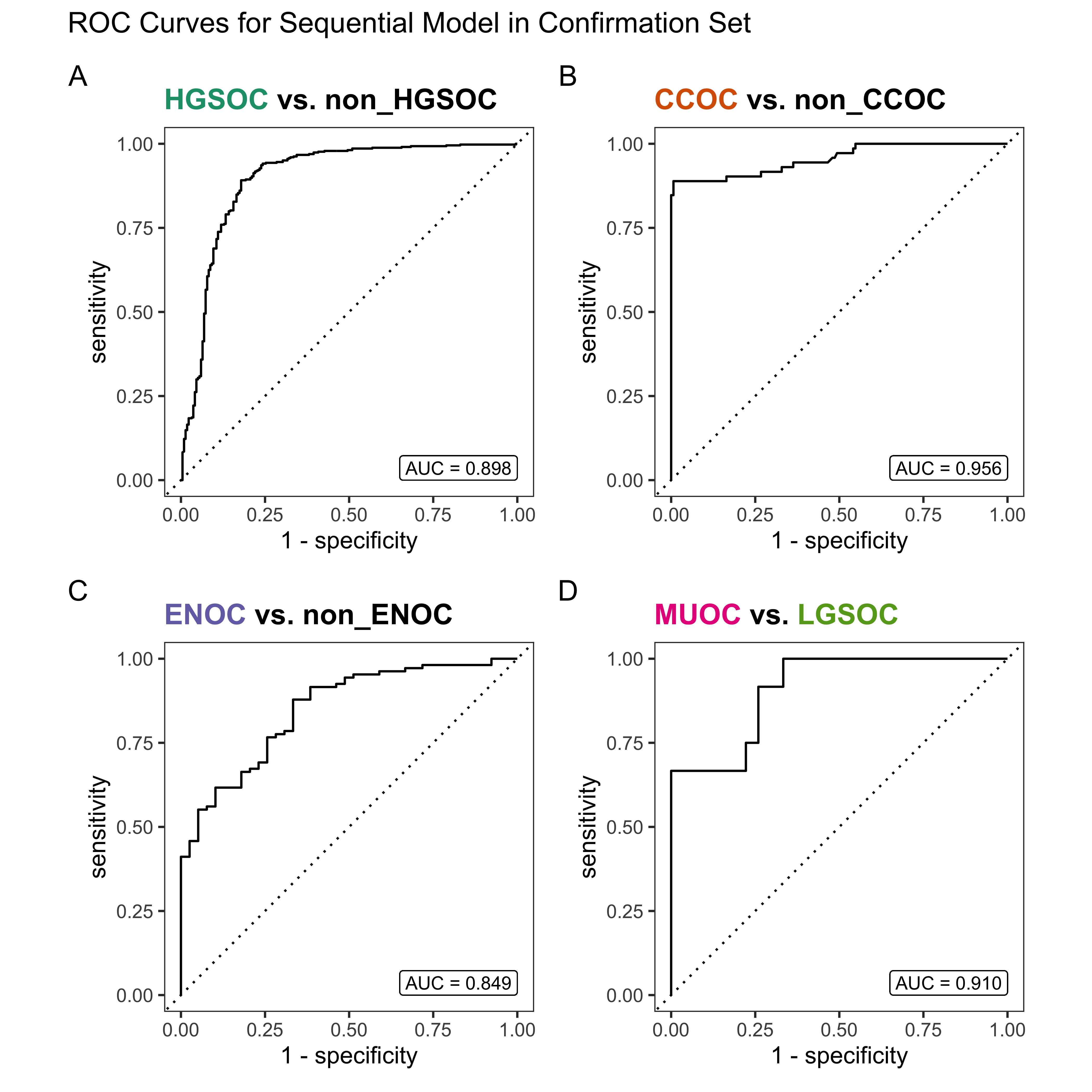
From Figure 4.9, we see that both Hybrid-XGB and SMOTE-SVM have the highest overall F1-Score and are relatively better at predicting the rarest histotype LGSOC (sensitivity = 0.42). Thus we choose both of these two workflows for gene optimization in the confirmation set. The optimal number of genes is determined by the highest average F1-Score across classes, including the overall metric in the average. We use an F1-score that is averaged across cross-validation folds (5) and class groups (6: Overall, HGSOC, CCOC, ENOC, MUOC, LGSOC) to compare performance between different number of genes selected.
4.4.1 Hybrid-XGB
In the Hybrid-XGB classifier, the optimal number of genes is highlighted in red in Figure 4.18. Hence the optimal number of total genes used will be n=28+19=47.
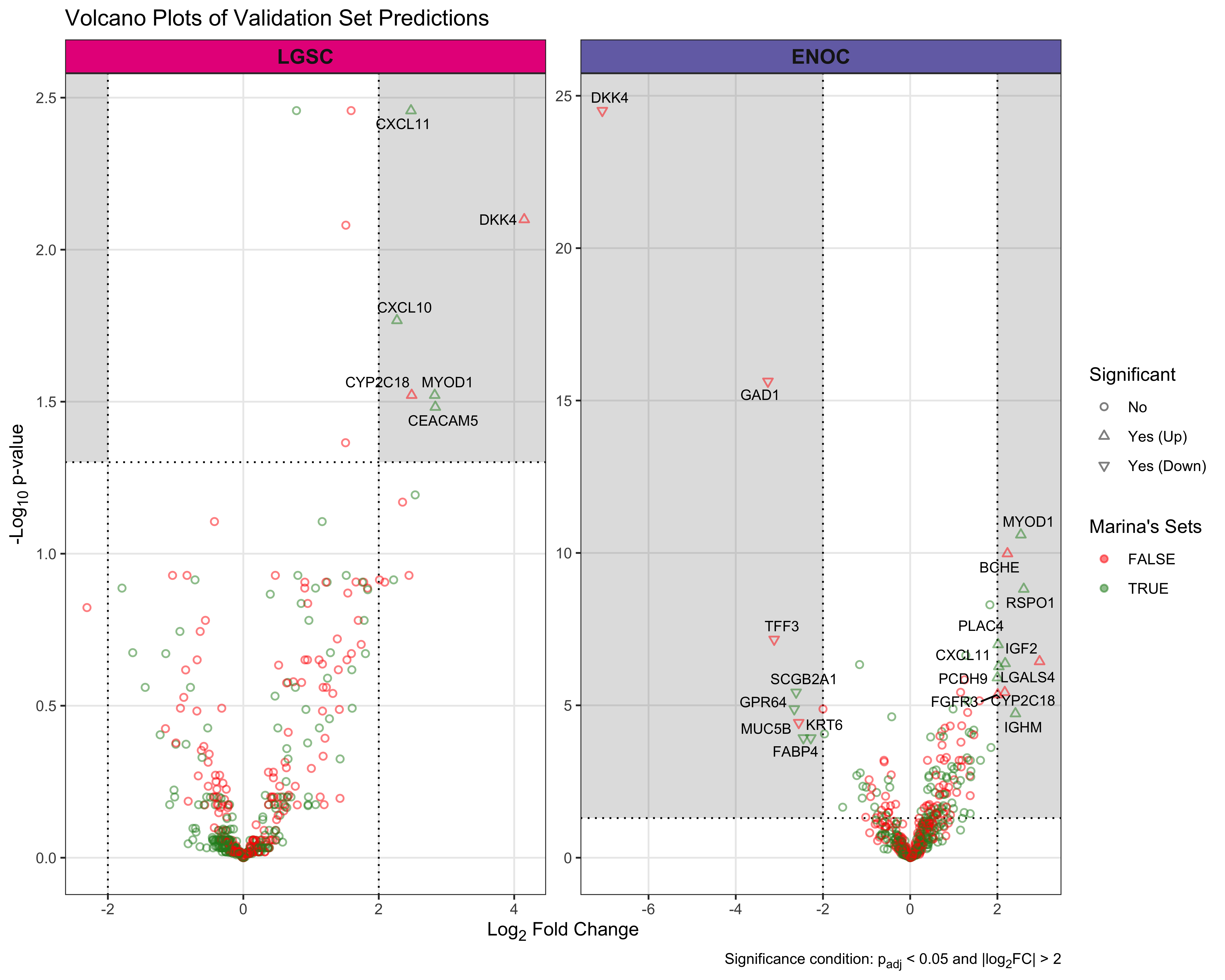
The gene profile of the optimal set of genes used is displayed in Table 4.15. Core genes in the PrOTYPE and SPOT sets are annotated with green circles, and the added genes are annotated with yellow circles. The added genes are: HNF1B, TFF1, TPX2, WT1, IGFBP1, LGALS4, TFF3, KLK7, CYP2C18, GPR64, CAPN2, MET, GCNT3, GAD1, SLC3A1, EGFL6, C1orf173, DKK4 and C10orf116. Unused genes are annotated with red crosses.
| Set | Genes | PrOTYPE | SPOT | Optimal Set | Candidate Rank |
|---|---|---|---|---|---|
| Core | COL11A1 | ✔ | ◉ | ||
| CD74 | ✔ | ◉ | |||
| CD2 | ✔ | ◉ | |||
| TIMP3 | ✔ | ◉ | |||
| LUM | ✔ | ◉ | |||
| CYTIP | ✔ | ◉ | |||
| COL3A1 | ✔ | ◉ | |||
| THBS2 | ✔ | ◉ | |||
| TCF7L1 | ✔ | ✔ | ◉ | ||
| HMGA2 | ✔ | ◉ | |||
| FN1 | ✔ | ◉ | |||
| POSTN | ✔ | ◉ | |||
| COL1A2 | ✔ | ◉ | |||
| COL5A2 | ✔ | ◉ | |||
| PDZK1IP1 | ✔ | ◉ | |||
| FBN1 | ✔ | ◉ | |||
| HIF1A | ✔ | ◉ | |||
| CXCL10 | ✔ | ◉ | |||
| DUSP4 | ✔ | ◉ | |||
| SOX17 | ✔ | ◉ | |||
| MITF | ✔ | ◉ | |||
| CDKN3 | ✔ | ◉ | |||
| BRCA2 | ✔ | ◉ | |||
| CEACAM5 | ✔ | ◉ | |||
| ANXA4 | ✔ | ◉ | |||
| SERPINE1 | ✔ | ◉ | |||
| CRABP2 | ✔ | ◉ | |||
| DNAJC9 | ✔ | ◉ | |||
| Candidates | HNF1B | ◉ | 1 | ||
| TFF1 | ◉ | 2 | |||
| TPX2 | ◉ | 3 | |||
| WT1 | ◉ | 4 | |||
| IGFBP1 | ◉ | 5 | |||
| LGALS4 | ◉ | 6 | |||
| TFF3 | ◉ | 7 | |||
| KLK7 | ◉ | 8 | |||
| CYP2C18 | ◉ | 9 | |||
| GPR64 | ◉ | 10 | |||
| CAPN2 | ◉ | 11 | |||
| MET | ◉ | 12 | |||
| GCNT3 | ◉ | 13 | |||
| GAD1 | ◉ | 14 | |||
| SLC3A1 | ◉ | 15 | |||
| EGFL6 | ◉ | 16 | |||
| C1orf173 | ◉ | 17 | |||
| DKK4 | ◉ | 18 | |||
| C10orf116 | ◉ | 19 | |||
| FUT3 | ⓧ | 20 | |||
| PBX1 | ⓧ | 21 | |||
| MUC5B | ⓧ | 22 | |||
| KGFLP2 | ⓧ | 23 | |||
| IGKC | ⓧ | 24 | |||
| IL6 | ⓧ | 25 | |||
| CPNE8 | ⓧ | 26 | |||
| CYP4B1 | ⓧ | 27 | |||
| TP53 | ⓧ | 28 | |||
| PAX8 | ⓧ | 29 | |||
| SERPINA5 | ⓧ | 30 | |||
| SENP8 | ⓧ | 31 | |||
| BRCA1 | ⓧ | 32 | |||
| STC1 | ⓧ | 33 | |||
| SEMA6A | ⓧ | 34 | |||
| TSPAN8 | ⓧ | 35 | |||
| LIN28B | ⓧ | 36 | |||
| EPAS1 | ⓧ | 37 | |||
| ATP5G3 | ⓧ | 38 | |||
| IGJ | ⓧ | 39 | |||
| SCGB1D2 | ⓧ | 40 | |||
| BCL2 | ⓧ | 41 | |||
| ADCYAP1R1 | ⓧ | 42 | |||
| MAP1LC3A | ⓧ | 43 |
4.4.2 SMOTE-SVM
In the SMOTE-svm classifier, the optimal number of genes is achieved at the highest averaged F1-score with 41 genes added, highlighted in red in Figure 4.19. Hence the optimal number of total genes used will be n=28+41=69.
The gene profile of the optimal set of genes used is displayed in Table 4.16. Core genes in the PrOTYPE and SPOT sets are annotated with green circles, and the added genes are annotated with yellow circles. The added genes are: EGFL6, IGJ, IGKC, TP53, DKK4, MUC5B, SLC3A1, MAP1LC3A, IGFBP1, CPNE8, SERPINA5, SCGB1D2, STC1, EPAS1, BRCA1, KGFLP2, SENP8, BCL2, PBX1, KLK7, C10orf116, LIN28B, LGALS4, ADCYAP1R1, IL6, ZBED1, WT1, TFF1, GCNT3, HNF1B, TFF3, CYP4B1, CYP2C18, TSPAN8, FUT3, MET, ATP5G3, SEMA6A, GPR64, PAX8 and C1orf173. Unused genes are annotated with red crosses.
| Set | Genes | PrOTYPE | SPOT | Optimal Set | Candidate Rank |
|---|---|---|---|---|---|
| Core | COL11A1 | ✔ | ◉ | ||
| CD74 | ✔ | ◉ | |||
| CD2 | ✔ | ◉ | |||
| TIMP3 | ✔ | ◉ | |||
| LUM | ✔ | ◉ | |||
| CYTIP | ✔ | ◉ | |||
| COL3A1 | ✔ | ◉ | |||
| THBS2 | ✔ | ◉ | |||
| TCF7L1 | ✔ | ✔ | ◉ | ||
| HMGA2 | ✔ | ◉ | |||
| FN1 | ✔ | ◉ | |||
| POSTN | ✔ | ◉ | |||
| COL1A2 | ✔ | ◉ | |||
| COL5A2 | ✔ | ◉ | |||
| PDZK1IP1 | ✔ | ◉ | |||
| FBN1 | ✔ | ◉ | |||
| HIF1A | ✔ | ◉ | |||
| CXCL10 | ✔ | ◉ | |||
| DUSP4 | ✔ | ◉ | |||
| SOX17 | ✔ | ◉ | |||
| MITF | ✔ | ◉ | |||
| CDKN3 | ✔ | ◉ | |||
| BRCA2 | ✔ | ◉ | |||
| CEACAM5 | ✔ | ◉ | |||
| ANXA4 | ✔ | ◉ | |||
| SERPINE1 | ✔ | ◉ | |||
| CRABP2 | ✔ | ◉ | |||
| DNAJC9 | ✔ | ◉ | |||
| Candidates | EGFL6 | ◉ | 1 | ||
| IGJ | ◉ | 2 | |||
| IGKC | ◉ | 3 | |||
| TP53 | ◉ | 4 | |||
| DKK4 | ◉ | 5 | |||
| MUC5B | ◉ | 6 | |||
| SLC3A1 | ◉ | 7 | |||
| MAP1LC3A | ◉ | 8 | |||
| IGFBP1 | ◉ | 9 | |||
| CPNE8 | ◉ | 10 | |||
| SERPINA5 | ◉ | 11 | |||
| SCGB1D2 | ◉ | 12 | |||
| STC1 | ◉ | 13 | |||
| EPAS1 | ◉ | 14 | |||
| BRCA1 | ◉ | 15 | |||
| KGFLP2 | ◉ | 16 | |||
| SENP8 | ◉ | 17 | |||
| BCL2 | ◉ | 18 | |||
| PBX1 | ◉ | 19 | |||
| KLK7 | ◉ | 20 | |||
| C10orf116 | ◉ | 21 | |||
| LIN28B | ◉ | 22 | |||
| LGALS4 | ◉ | 23 | |||
| ADCYAP1R1 | ◉ | 24 | |||
| IL6 | ◉ | 25 | |||
| ZBED1 | ◉ | 26 | |||
| WT1 | ◉ | 27 | |||
| TFF1 | ◉ | 28 | |||
| GCNT3 | ◉ | 29 | |||
| HNF1B | ◉ | 30 | |||
| TFF3 | ◉ | 31 | |||
| CYP4B1 | ◉ | 32 | |||
| CYP2C18 | ◉ | 33 | |||
| TSPAN8 | ◉ | 34 | |||
| FUT3 | ◉ | 35 | |||
| MET | ◉ | 36 | |||
| ATP5G3 | ◉ | 37 | |||
| SEMA6A | ◉ | 38 | |||
| GPR64 | ◉ | 39 | |||
| PAX8 | ◉ | 40 | |||
| C1orf173 | ◉ | 41 | |||
| GAD1 | ⓧ | 42 | |||
| CAPN2 | ⓧ | 43 |
4.4.3 Gene List Comparisons in Confirmation Set
We train the Hybrid-XGB and SMOTE-SVM workflows using the core and optimal gene lists in the training set. The models are evaluated on the confirmation set. Overall and per-class results are shown in Table 4.17. The gene lists are:
Core (n=28): among the overlapping genes, the core set from the PrOTYPE and SPOT lists
Optimal (n=47, 69): among the overlapping genes, the core set plus the additional number of genes that result in the optimal value for a selected evaluation metric, as assessed in Figure 4.18 and Figure 4.19
| Method | Metric | Overall | HGSOC | CCOC | ENOC | MUOC | LGSOC |
|---|---|---|---|---|---|---|---|
| Hybrid-XGB, Optimal | Accuracy | 0.836 | 0.872 | 0.966 | 0.893 | 0.966 | 0.977 |
| Sensitivity | 0.694 | 0.946 | 0.861 | 0.458 | 0.704 | 0.500 | |
| Specificity | 0.930 | 0.729 | 0.979 | 0.979 | 0.977 | 0.986 | |
| F1-Score | 0.684 | 0.907 | 0.849 | 0.587 | 0.633 | 0.444 | |
| Balanced Accuracy | 0.812 | 0.838 | 0.920 | 0.719 | 0.840 | 0.743 | |
| Kappa | 0.670 | 0.703 | 0.830 | 0.531 | 0.616 | 0.433 | |
| Hybrid-XGB, Core | Accuracy | 0.810 | 0.858 | 0.952 | 0.872 | 0.970 | 0.967 |
| Sensitivity | 0.613 | 0.929 | 0.875 | 0.393 | 0.704 | 0.167 | |
| Specificity | 0.923 | 0.720 | 0.961 | 0.968 | 0.982 | 0.983 | |
| F1-Score | 0.606 | 0.896 | 0.803 | 0.506 | 0.667 | 0.160 | |
| Balanced Accuracy | 0.768 | 0.825 | 0.918 | 0.680 | 0.843 | 0.575 | |
| Kappa | 0.620 | 0.673 | 0.775 | 0.440 | 0.651 | 0.143 | |
| SMOTE-SVM, Optimal | Accuracy | 0.821 | 0.860 | 0.958 | 0.879 | 0.974 | 0.972 |
| Sensitivity | 0.666 | 0.932 | 0.847 | 0.458 | 0.593 | 0.500 | |
| Specificity | 0.925 | 0.720 | 0.972 | 0.963 | 0.990 | 0.981 | |
| F1-Score | 0.665 | 0.898 | 0.819 | 0.557 | 0.653 | 0.400 | |
| Balanced Accuracy | 0.796 | 0.826 | 0.910 | 0.710 | 0.791 | 0.740 | |
| Kappa | 0.640 | 0.676 | 0.795 | 0.490 | 0.639 | 0.386 | |
| SMOTE-SVM, Core | Accuracy | 0.815 | 0.860 | 0.952 | 0.874 | 0.970 | 0.974 |
| Sensitivity | 0.672 | 0.903 | 0.889 | 0.514 | 0.556 | 0.500 | |
| Specificity | 0.930 | 0.775 | 0.960 | 0.946 | 0.989 | 0.983 | |
| F1-Score | 0.660 | 0.895 | 0.805 | 0.576 | 0.612 | 0.414 | |
| Balanced Accuracy | 0.801 | 0.839 | 0.924 | 0.730 | 0.772 | 0.741 | |
| Kappa | 0.641 | 0.685 | 0.778 | 0.503 | 0.597 | 0.401 |
4.5 Validation Set
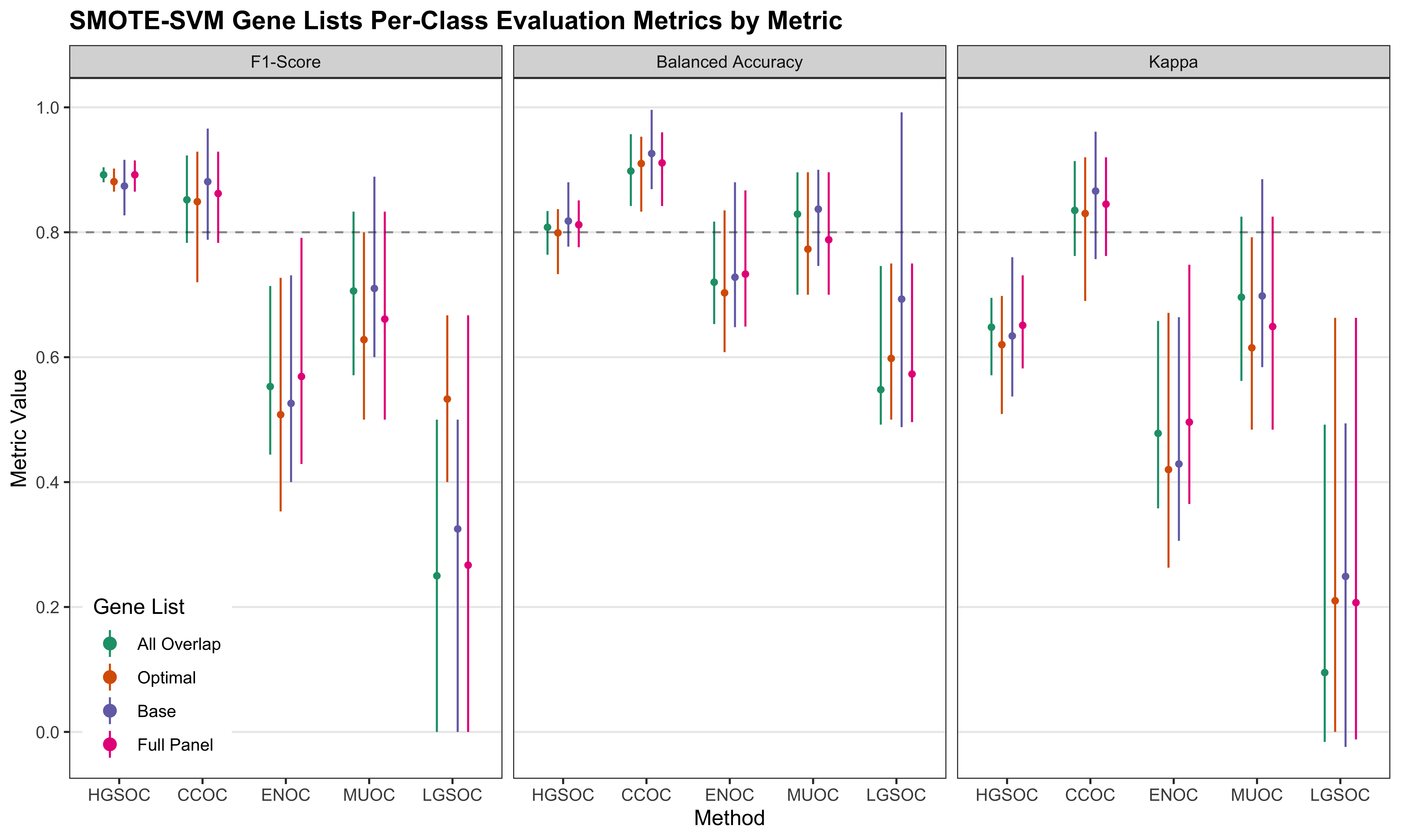
From the results in Table 4.17 and Figure 4.20, we see that the Hybrid-XGB, optimal workflow as the highest overall F1-Score and balanced accuracy. Thus, we choose the Hybrid-XGB model trained on the training set for the all overlap, optimal, and core gene lists, and evaluate performance in the validation set.
4.5.1 Evaluation Metrics
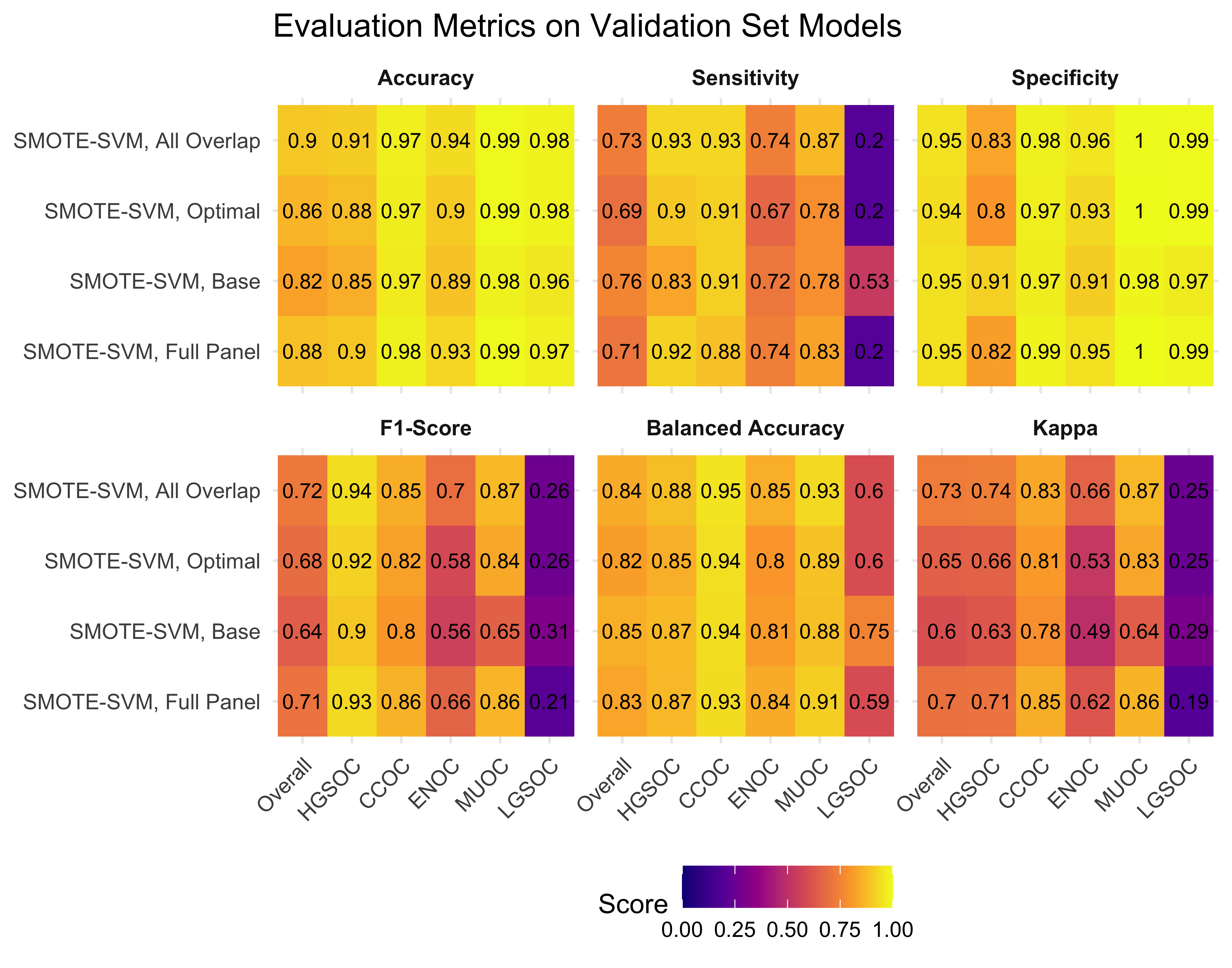
| Method | Metric | Overall | HGSOC | CCOC | ENOC | MUOC | LGSOC |
|---|---|---|---|---|---|---|---|
| Hybrid-XGB, All Overlap | Accuracy | 0.889 | 0.905 | 0.969 | 0.955 | 0.978 | 0.972 |
| Sensitivity | 0.799 | 0.913 | 1.000 | 0.682 | 0.870 | 0.533 | |
| Specificity | 0.958 | 0.877 | 0.966 | 0.985 | 0.980 | 0.980 | |
| F1-Score | 0.715 | 0.938 | 0.831 | 0.750 | 0.667 | 0.390 | |
| Balanced Accuracy | 0.879 | 0.895 | 0.983 | 0.833 | 0.925 | 0.756 | |
| Kappa | 0.725 | 0.739 | 0.815 | 0.726 | 0.656 | 0.377 | |
| Hybrid-XGB, Optimal | Accuracy | 0.876 | 0.894 | 0.966 | 0.949 | 0.974 | 0.969 |
| Sensitivity | 0.789 | 0.904 | 0.971 | 0.625 | 0.913 | 0.533 | |
| Specificity | 0.952 | 0.856 | 0.966 | 0.984 | 0.976 | 0.976 | |
| F1-Score | 0.692 | 0.930 | 0.817 | 0.705 | 0.646 | 0.364 | |
| Balanced Accuracy | 0.870 | 0.880 | 0.969 | 0.804 | 0.944 | 0.755 | |
| Kappa | 0.694 | 0.709 | 0.799 | 0.677 | 0.634 | 0.349 | |
| Hybrid-XGB, Core | Accuracy | 0.843 | 0.877 | 0.954 | 0.923 | 0.966 | 0.966 |
| Sensitivity | 0.721 | 0.897 | 0.942 | 0.386 | 0.913 | 0.467 | |
| Specificity | 0.937 | 0.805 | 0.955 | 0.981 | 0.968 | 0.975 | |
| F1-Score | 0.615 | 0.919 | 0.760 | 0.496 | 0.583 | 0.318 | |
| Balanced Accuracy | 0.829 | 0.851 | 0.949 | 0.684 | 0.940 | 0.721 | |
| Kappa | 0.611 | 0.661 | 0.736 | 0.458 | 0.568 | 0.303 |
4.5.2 Confusion Matrices
4.5.3 ROC Curves
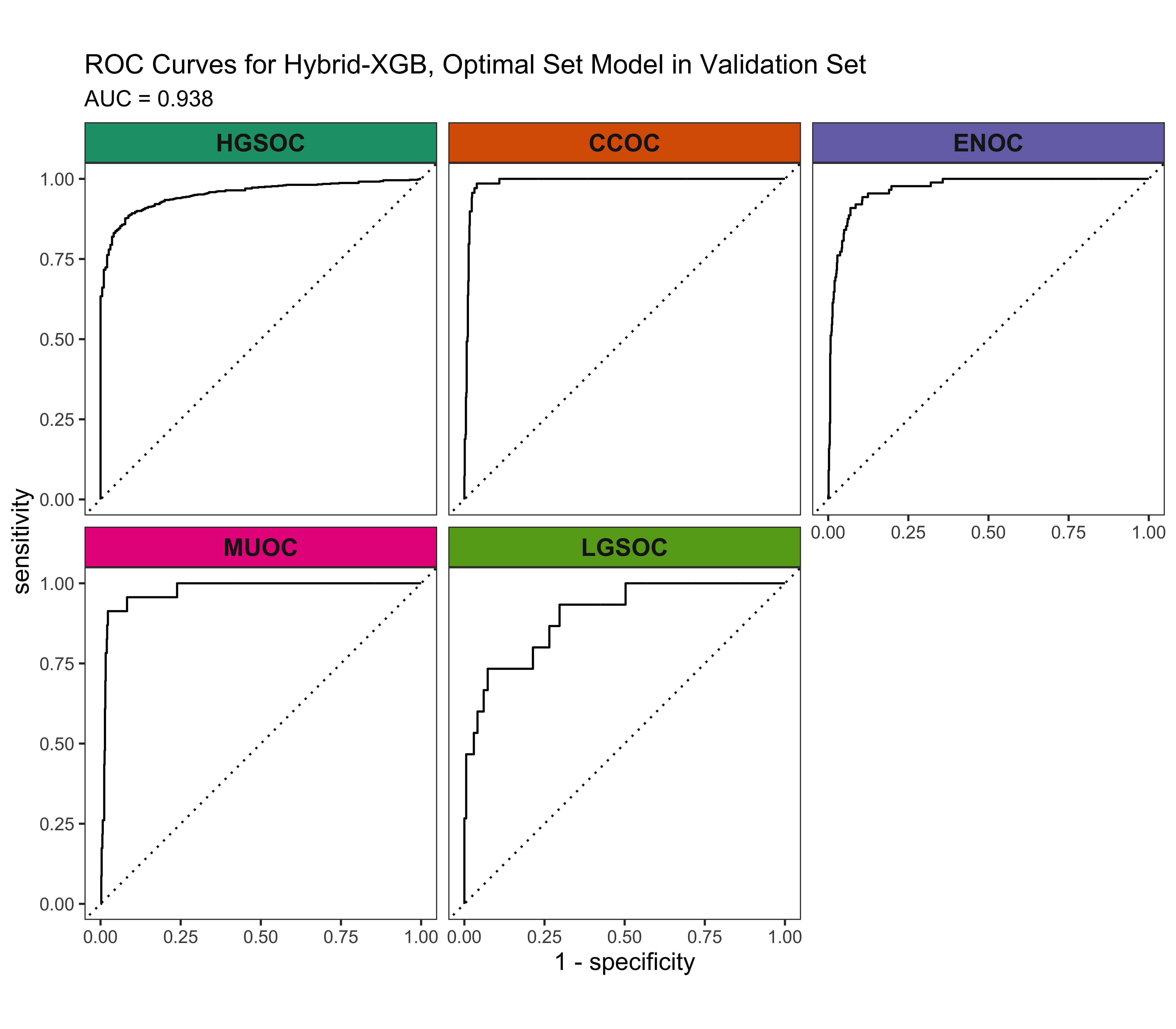
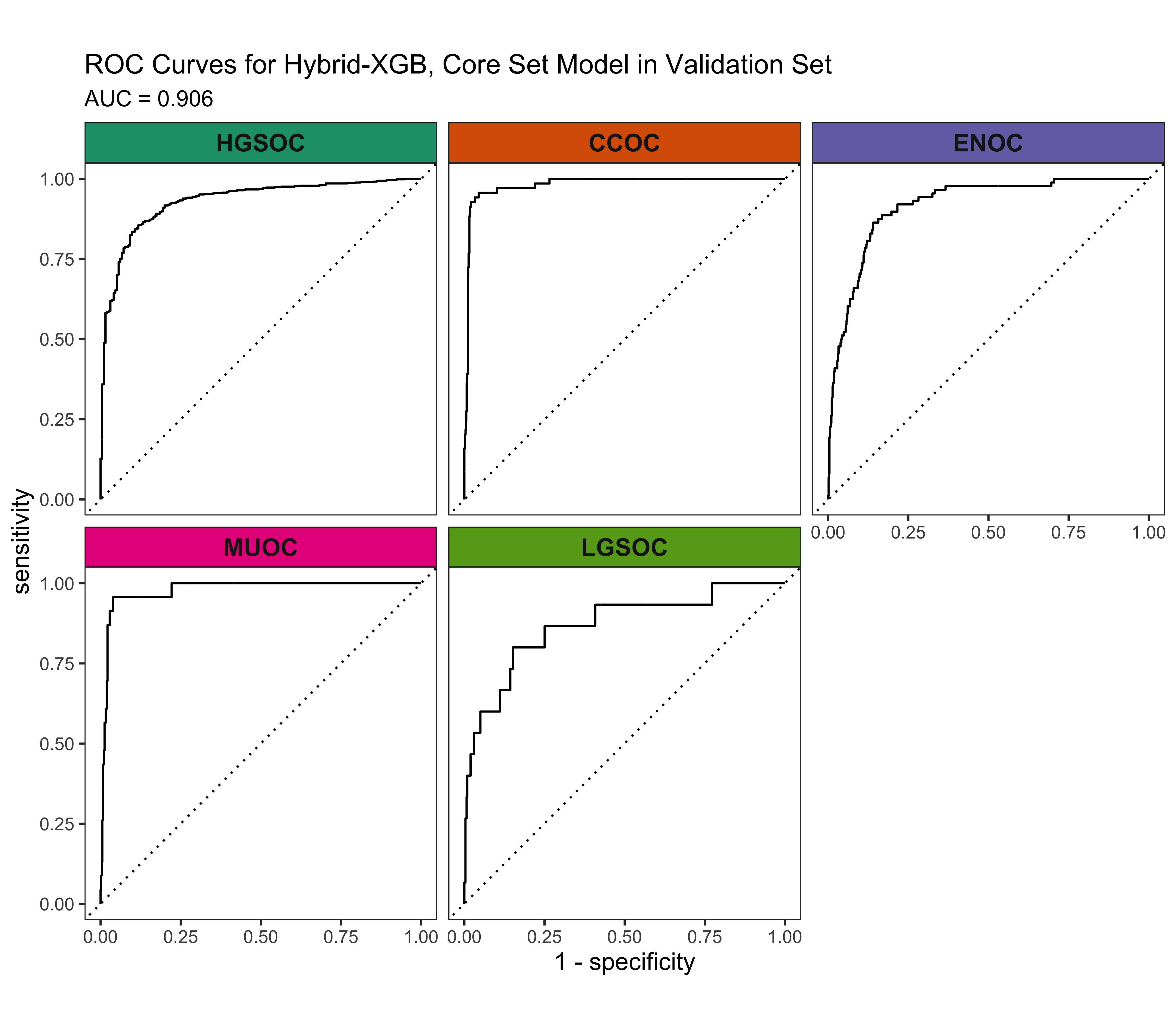
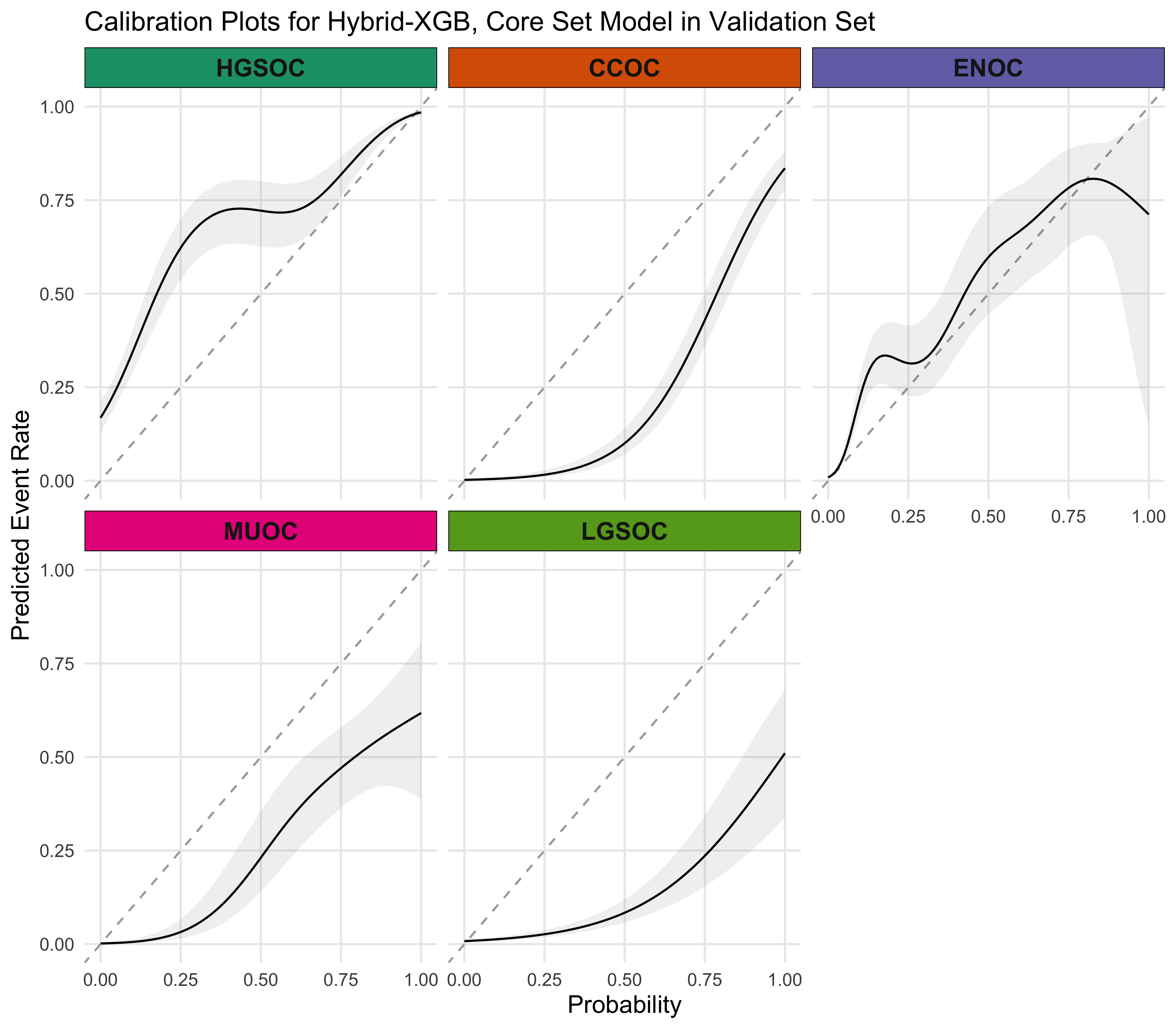
4.5.4 Calibration Plots
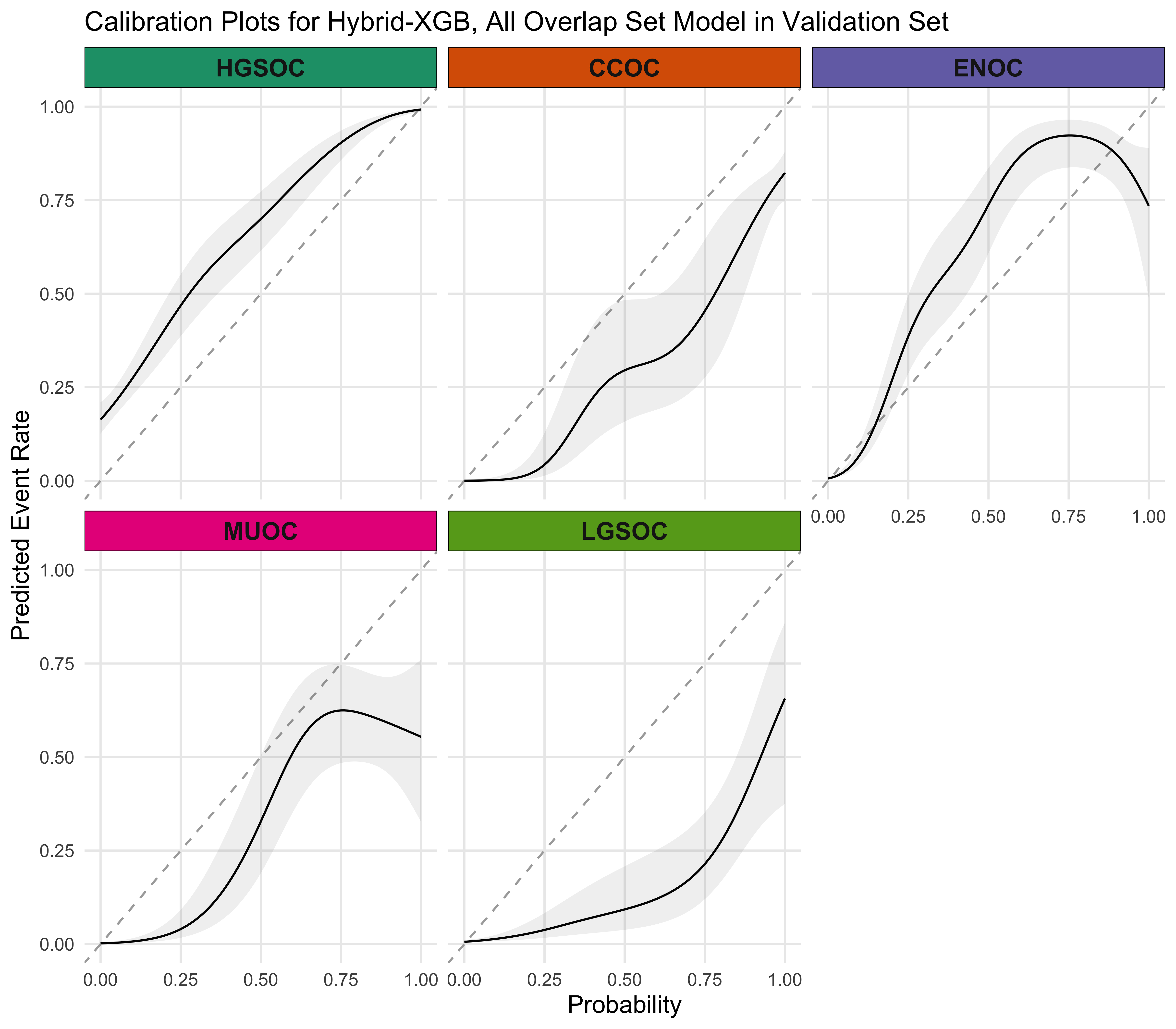
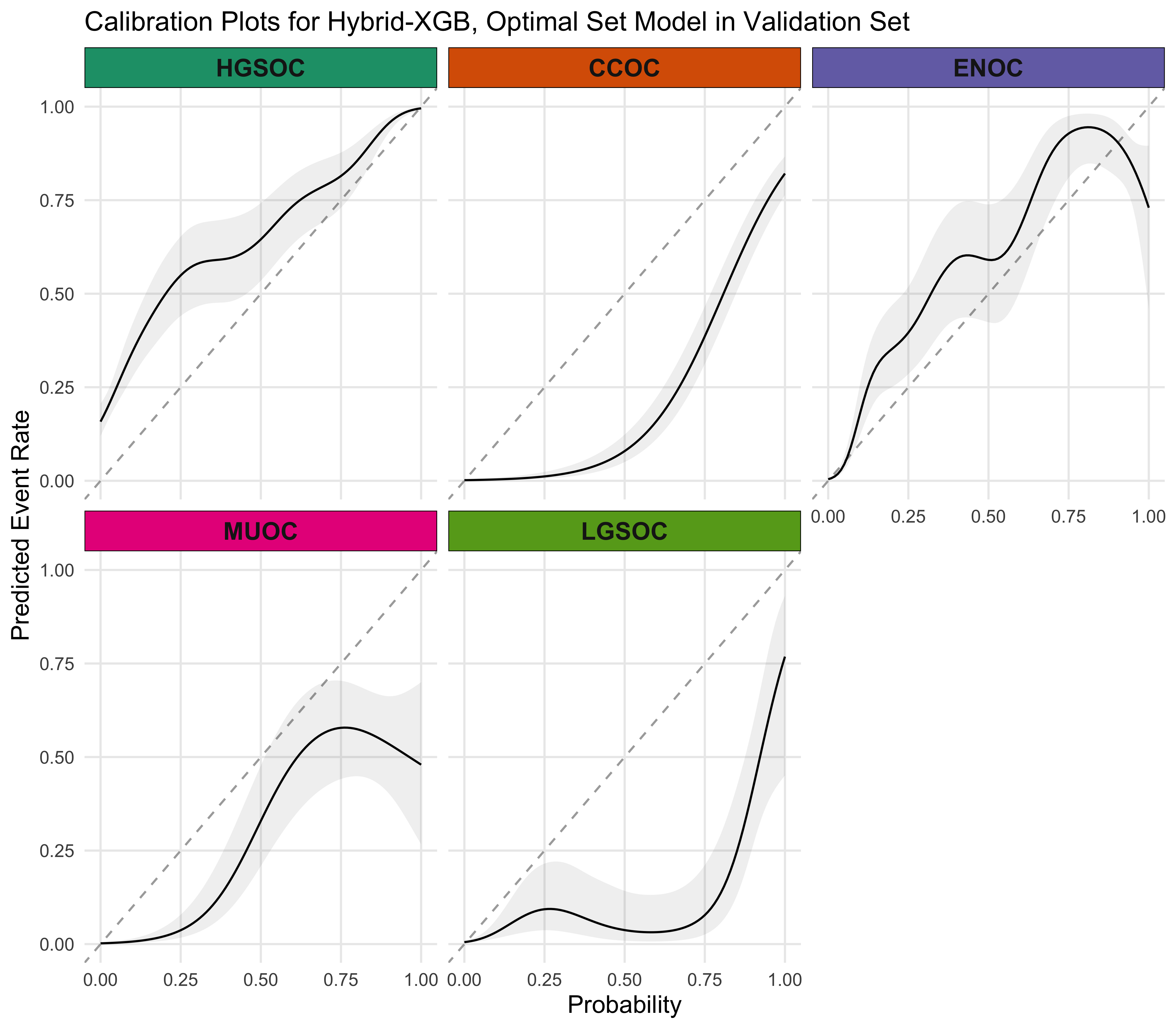
4.5.5 Final Model
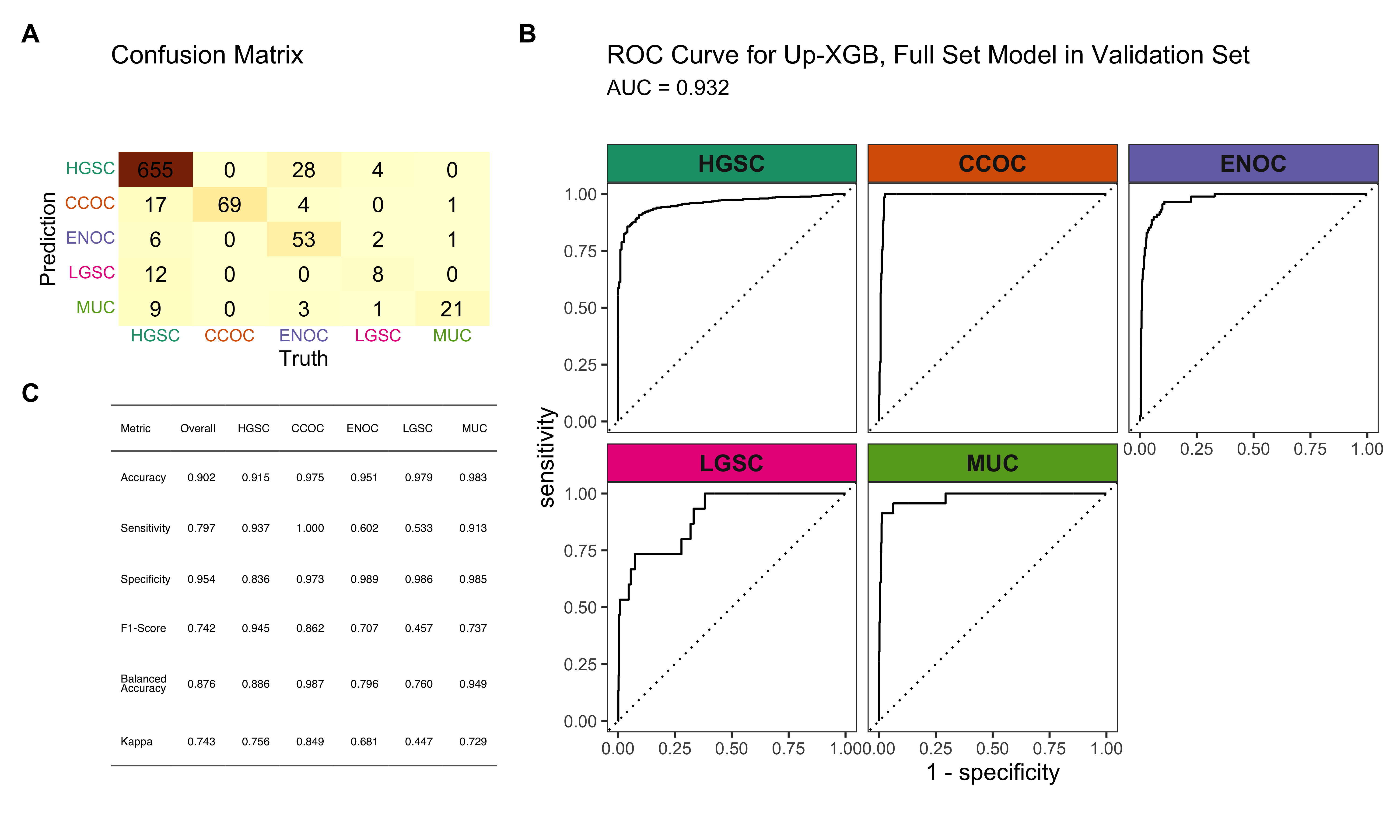
A summary of the Hybrid-XGB, Optimal model results are shown in Figure 4.29.
4.5.5.1 Feature Importance
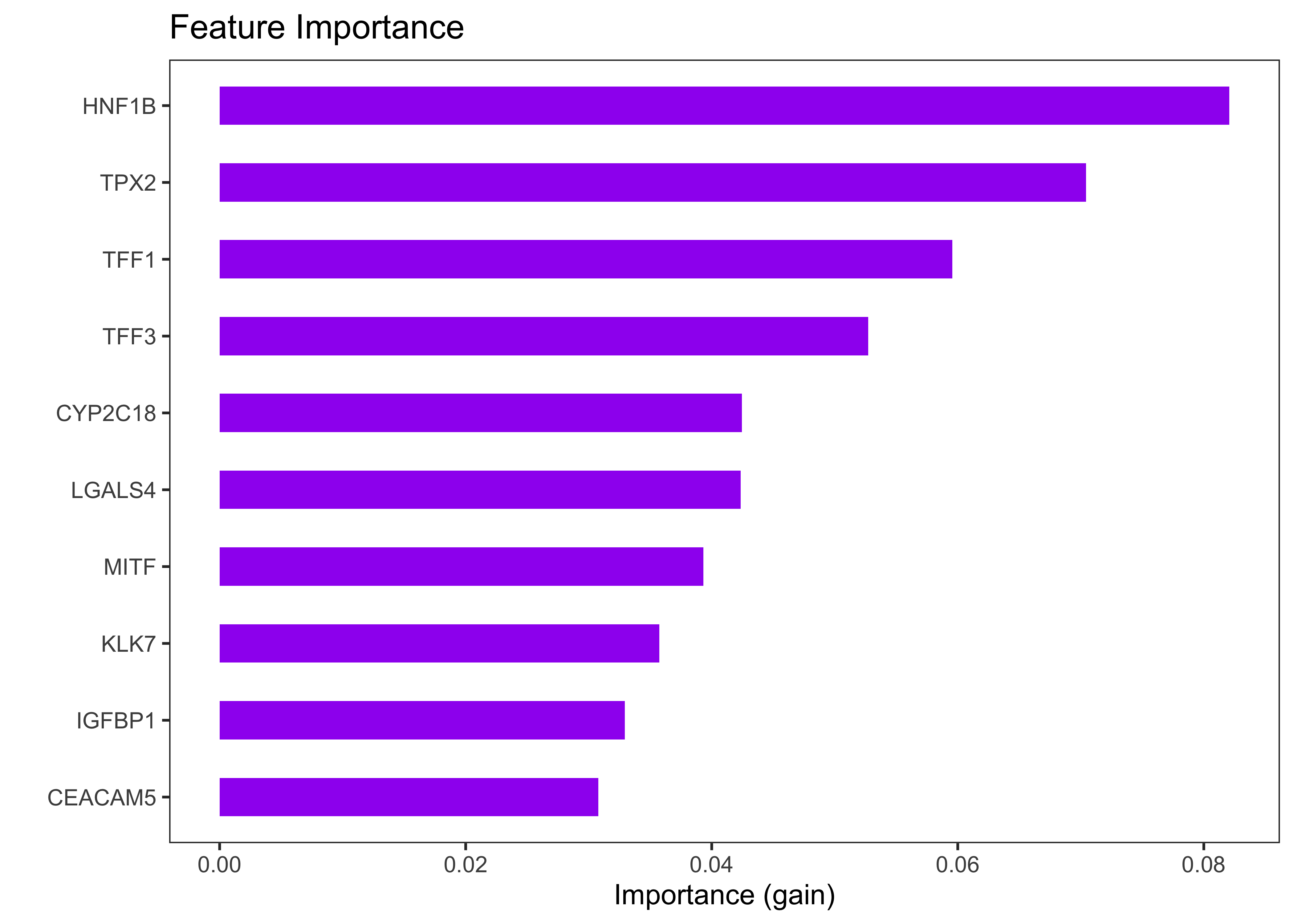
For a tree model, the “gain” is the most frequently used variable importance measure. It represents the fractional contribution of each feature to the model based on the total gain of this feature’s splits. A higher percentage means higher importance. Figure Figure 4.30 shows the gain for the top 10 features of the final model (Hybrid-XGB).
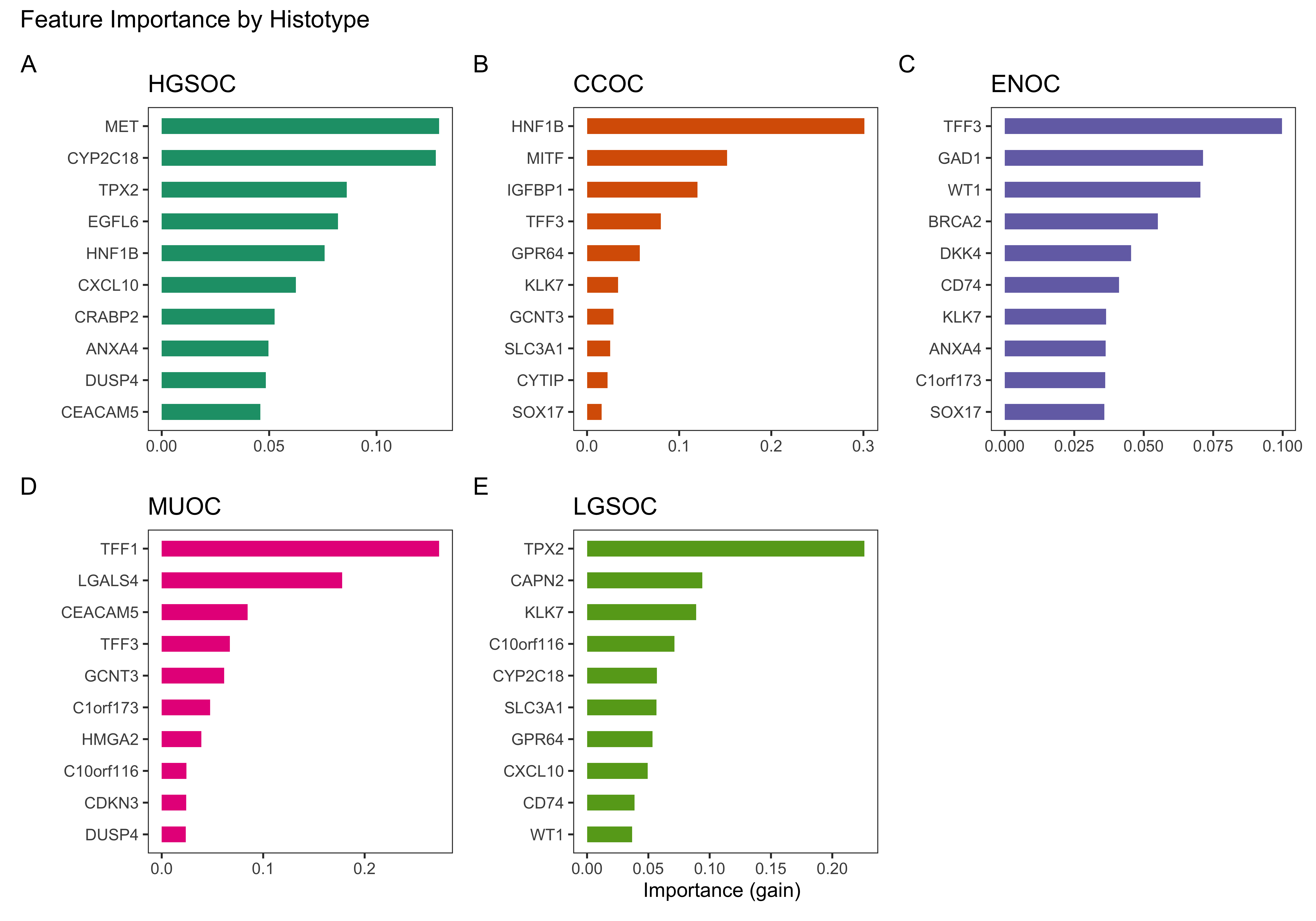
XGBoost builds a separate set of trees sequentially during each boosting round. We are able to calculate variable importance for each of the histotypes by including only the trees that are associated with their class index.
For example, the class index labels from our model are ordered CCOC, ENOC, HGSOC, LGSOC, MUOC. Assuming a total of 214 boosting rounds, every 5th tree is selected using these indices:
CCOC: 1, 6, 11, …, 1066
ENOC: 2, 7, 12, …, 1067
HGSOC: 3, 8, 13, …, 1068
LGSOC: 4, 9, 14, …, 1069
MUOC: 5, 10, 15, …, 1070
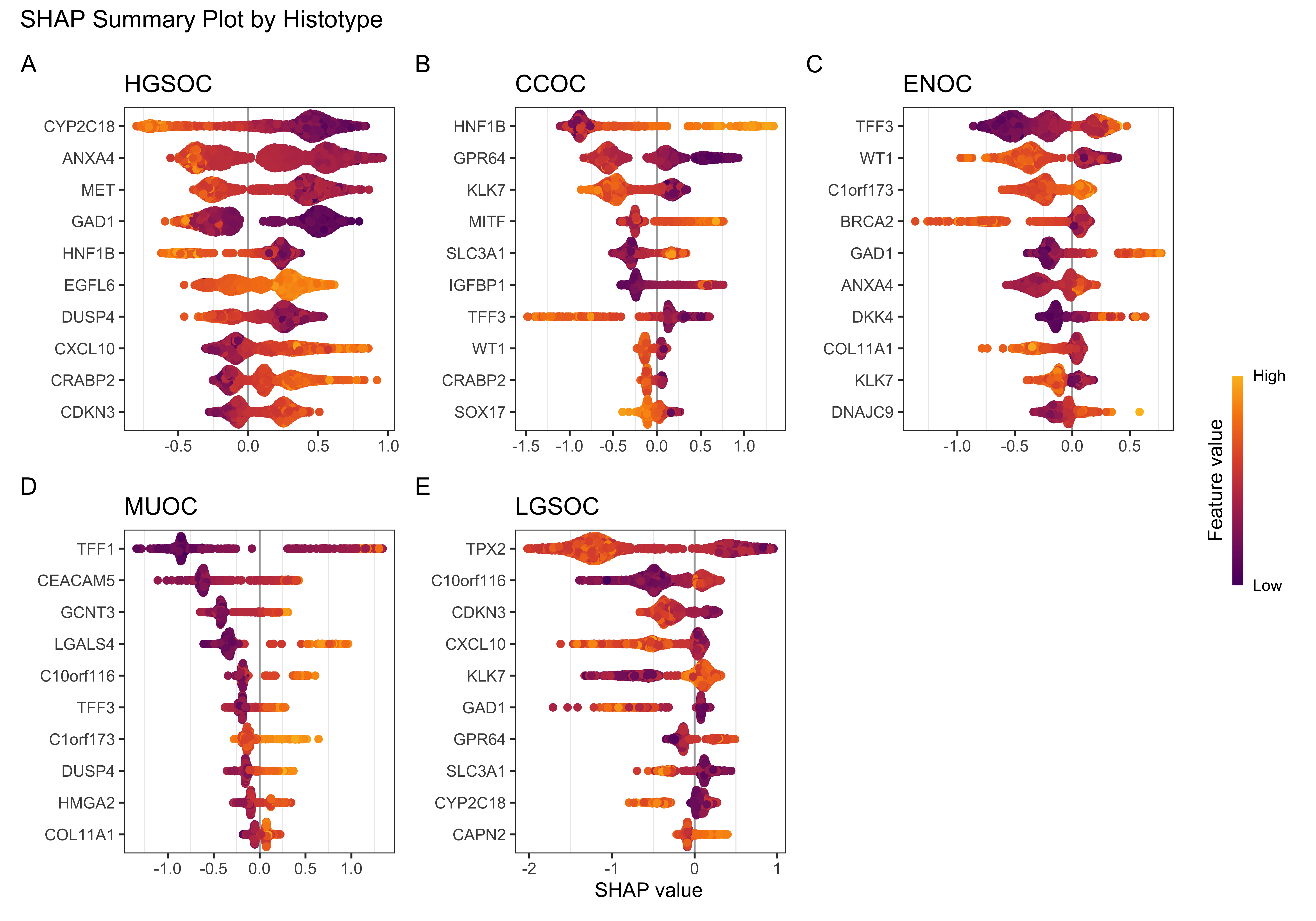
A SHAP importance plot incorporates directionality and distribution of the importance patterns (Lundberg and Lee 2017). Figure Figure 4.32 illustrates a beeswarm plot for each histotype. We only show the top 10 features, with the most important at the top to the least important at the bottom. Positive SHAP values increase the prediction and negative SHAP values decrease the prediction. The colours represent feature values, with low values coloured purple and high values coloured yellow. Finally, the density of the points indicate whether there is a high concentration of observations distributed at a particular SHAP value.
For example, we see that for CCOC, higher values of the gene HNF1B increase the prediction and lower values decrease the prediction. Conversely, lower values of CYP2C18 decrease the prediction of HGSOC and vice versa.
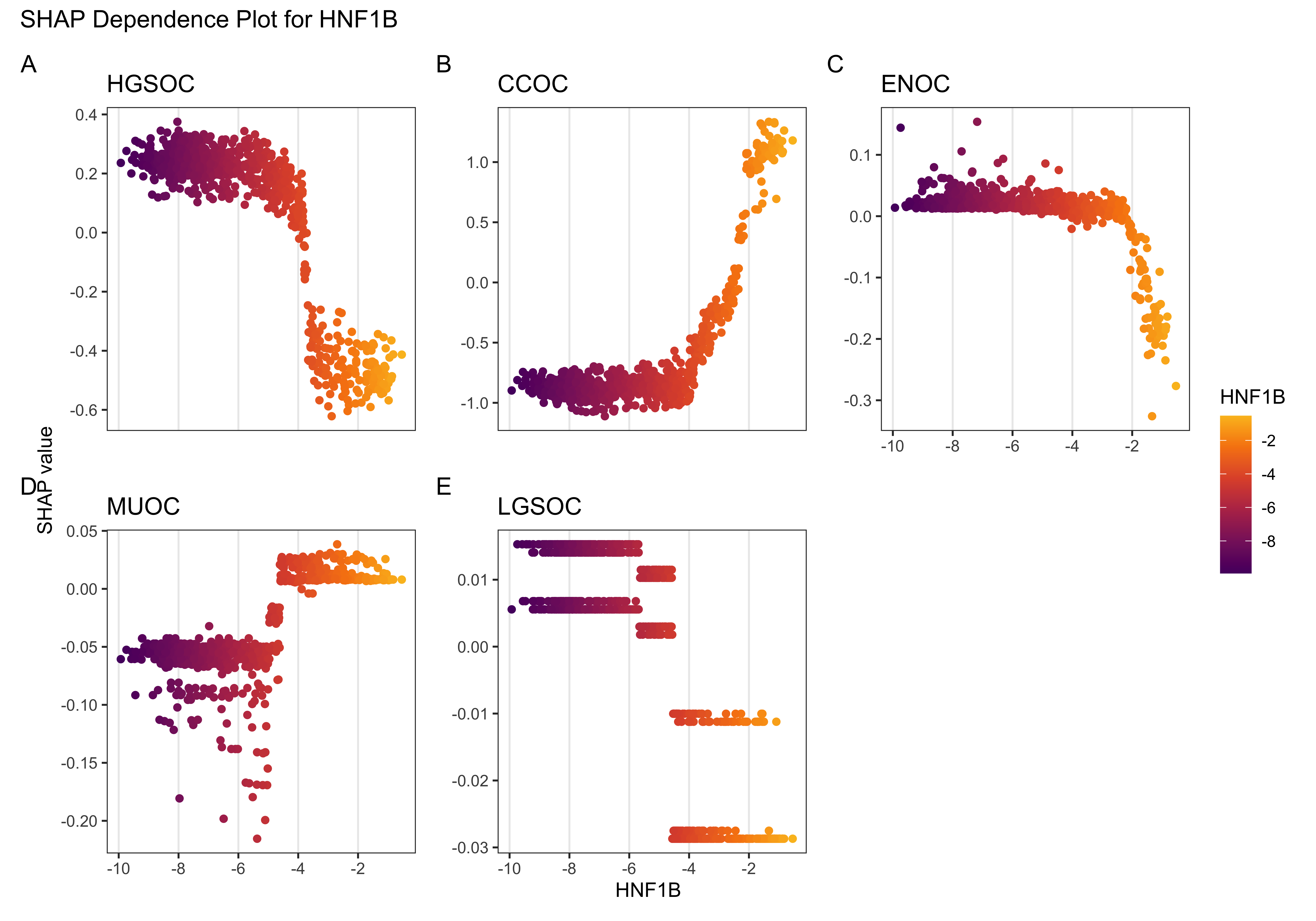
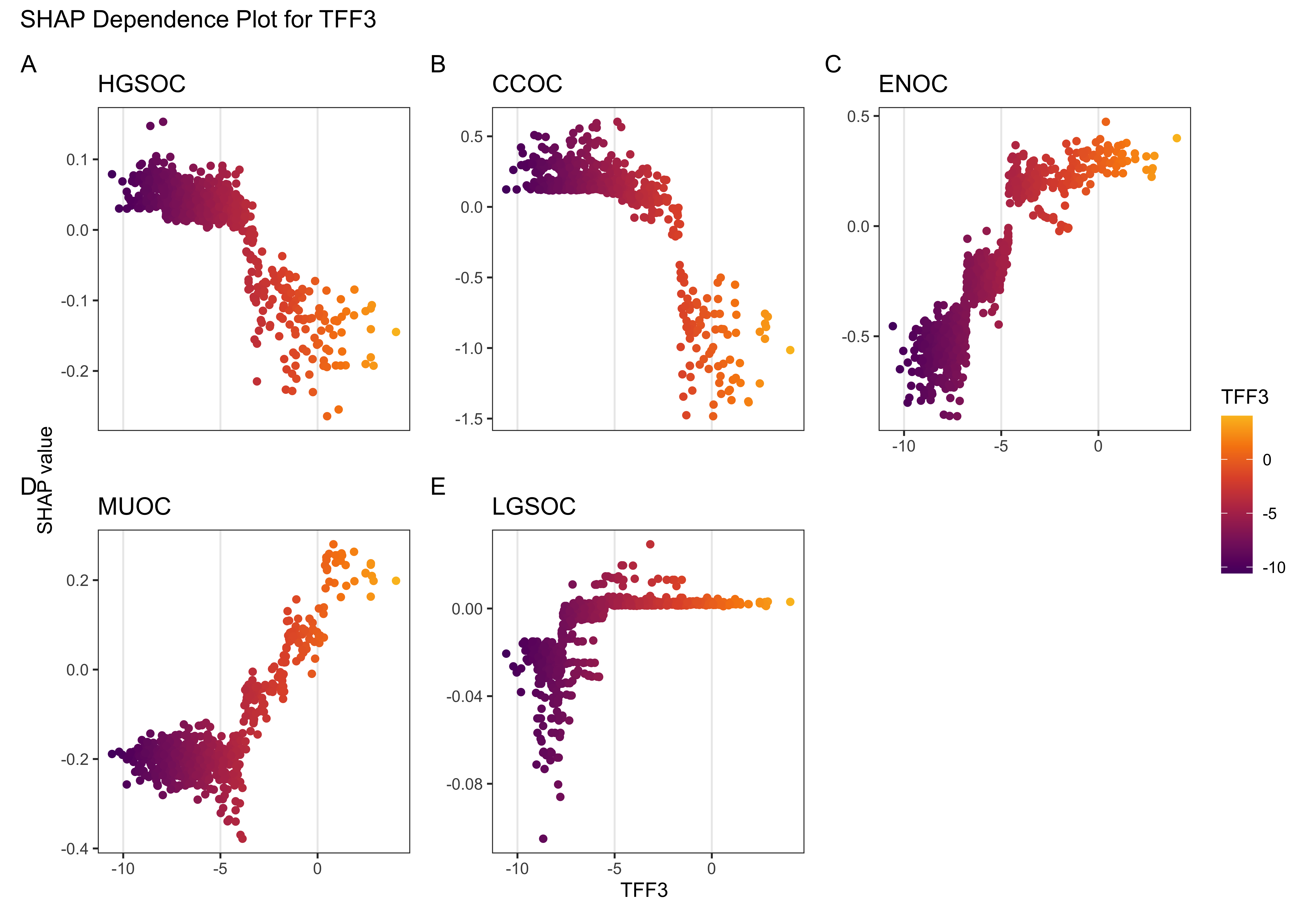
We can use a scatterplot to visualize how the actual values of individual features affect SHAP values, and subsequently the model predictions. The relationship may be linear, curved, or some other complex pattern. Fig Figure 4.33 and Figure 4.34 show the SHAP dependence plots for HNF1B and TFF3 respectively.
We know from the beeswarm plot that HNF1B was the most important feature for the CCOC class. SHAP values are relatively flat until HNF1B increases past -4, at which point the SHAP values start to increase sharply and prediction is strongly driven toward CCOC. At the same value of -4, the inverse pattern is observed for HGSOC.
TFF3 was the most important feature for ENOC prediction. SHAP values start to flip to positive after TFF3 increases past -5. On the other hand for CCOC, SHAP values start to flip to negative as TFF3 increases past -2, driving prediction away from the CCOC class.
4.5.5.2 Gene Membership
4.5.6 Additional Explorations
| Characteristic | Predicted ENOC Correctly N = 551 |
Missed ENOC N = 331 |
p-value2 |
|---|---|---|---|
| Age at diagnosis | 53 (46, 63) | 56 (51, 62) | 0.3 |
| Tumour grade | 0.003 | ||
| low grade | 42 (93%) | 17 (63%) | |
| high grade | 3 (6.7%) | 10 (37%) | |
| Unknown | 10 | 6 | |
| FIGO tumour stage | 0.086 | ||
| I | 42 (78%) | 20 (61%) | |
| II-IV | 12 (22%) | 13 (39%) | |
| Unknown | 1 | 0 | |
| Race | 0.7 | ||
| white | 50 (93%) | 26 (90%) | |
| non-white | 4 (7.4%) | 3 (10%) | |
| Unknown | 1 | 4 | |
| ARID1A | >0.9 | ||
| absent/subclonal | 10 (18%) | 6 (18%) | |
| present | 45 (82%) | 27 (82%) | |
| WT1 | 0.3 | ||
| diffuse (>50%) | 2 (3.6%) | 3 (9.1%) | |
| focal (1-50%) | 3 (5.5%) | 0 (0%) | |
| negative | 50 (91%) | 30 (91%) | |
| TP53 | 0.059 | ||
| mutated | 1 (1.8%) | 4 (13%) | |
| wild type | 54 (98%) | 28 (88%) | |
| Unknown | 0 | 1 | |
| PR | 0.010 | ||
| diffuse (>50%) | 35 (64%) | 11 (33%) | |
| focal (1-50%) | 9 (16%) | 6 (18%) | |
| negative | 11 (20%) | 16 (48%) | |
| P16 | 0.10 | ||
| abnormal block | 2 (3.6%) | 4 (12%) | |
| abnormal complete absence | 13 (24%) | 12 (36%) | |
| normal | 40 (73%) | 17 (52%) | |
| NAPSIN A | 0.5 | ||
| negative | 53 (96%) | 32 (100%) | |
| positive | 2 (3.6%) | 0 (0%) | |
| Unknown | 0 | 1 | |
| 1 Median (Q1, Q3); n (%) | |||
| 2 Wilcoxon rank sum test; Fisher’s exact test; Pearson’s Chi-squared test | |||