The nanostringr R package is a companion R package to
the manuscript:
A. Talhouk, S. Kommoss, R. Mackenzie, M. Cheung, S. Leung, D. Chiu, S. Kalloger, D. Huntsman, S. Chen, M. Intermaggio, J. Gronwald, F. Chan, S. Ramus, C. Steidl, D. Scott, M. Anglesio. (2016). Single-patient molecular testing with NanoString nCounter Data using a reference-based strategy for batch effect correction. PLos ONE.
This vignette provides a guide to reproduce the analyses in the paper and document the use of some of the functions.
The Data
Included in this package are several datasets that are described in detail in the manuscript and that are annotated in expQC, the annotation data frame for all of the experiments, run in different CodeSets, including:
-
Hodgkin Lymphoma Clinical Samples (HL) TOTAL 74
samples
- HL1 n=32 Unique Samples
- HL2 n=32 Replicates of HL1 samples
- HL3 n=10 Replicates (subset of HL1 samples)
-
Ovarian Cancer Clinical Samples (OC) TOTAL 258
samples
- OC1 n=129 Unique
- OC2 n=129 Replicates of OC1 samples
-
Ovarian Cancer Cell Lines (OVCL) TOTAL 26 samples
- OC1 n=13 Unique
- OC2 n=13 Replicates of OC1 samples
-
DNA Oligonucleotides for the HL CodeSet (HLO) TOTAL
68 HLO pool run at different concentrations
- HL1 n=36
- HL2 n=30
- HL3 n=2
- HL1 n=36
-
DNA Oligonucleotides for the OC CodeSet (OVO) TOTAL
135 OVO pool run at different concentrations
- OC1 n=47
- OC2 n=88
- OC1 n=47
The Functions
NanoStringQC
The NanoStringQC function computes several QC metrics and appends them to the annotation matrix. Care should be taken to ensure that the data is in the proper format. The function returns different QC metric flags that can be used to filter out samples that fail QC.
library(nanostringr)
expOVD <- NanoStringQC(ovd.r, subset(expQC, OVD == "Yes"))
expOVO <- NanoStringQC(ovo.r, subset(expQC, OVO == "Yes"))
expOVCL <- NanoStringQC(ovc.r, subset(expQC, OVCL == "Yes"))
expHLD <- NanoStringQC(hld.r, subset(expQC, HLD == "Yes"))
expHLO <- NanoStringQC(hlo.r, subset(expQC, HLO == "Yes"))
expQC <- rbind(expHLD, expOVD, expHLO, expOVO, expOVCL)
expQC$cohort <- factor(
  x = c(
    rep("HLD", nrow(expHLD)),
    rep("OVD", nrow(expOVD)),
    rep("HLO", nrow(expHLO)),
    rep("OVO", nrow(expOVO)),
    rep("OVCL", nrow(expOVCL))
  ),
  levels = c("HLD", "OVD", "OVCL", "HLO", "OVO"),
  labels = c("HL", "OC", "OVCL", "HLO", "OVO")
)Fields Of View (FOV)
boxplot(perFOV ~ cohort, ylab = "% FOV", main = "% FOV by Cohort", data = expQC, pch = 20,
        col = c(COL.HLD, COL.OVD, COL.OVCL, COL.HLO, COL.OVO))
abline(h = 75, lty = 2, col = "red")
grid(NULL, NULL, lwd = 1)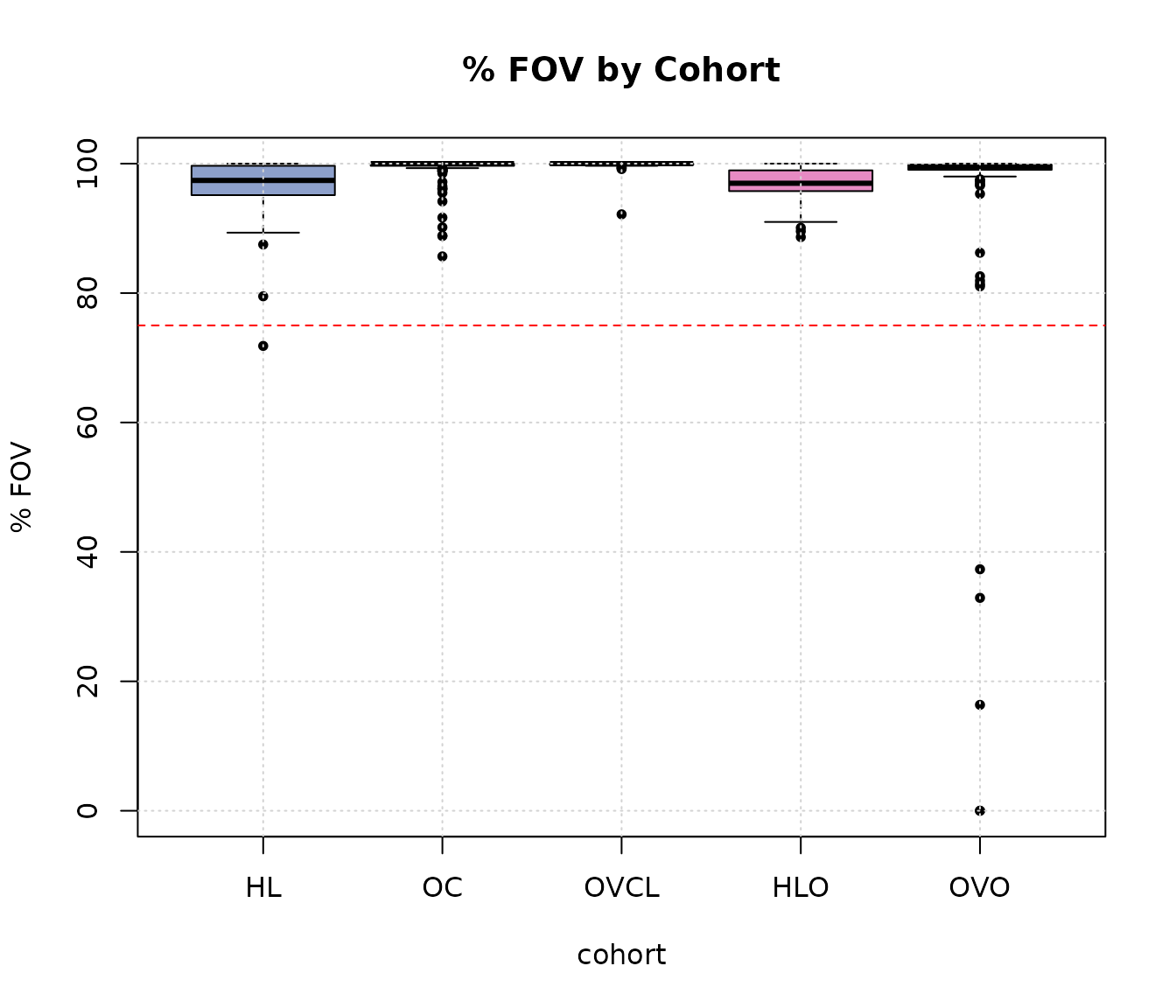
Samples that failed imaging QC based on percent fields of view (FOV) counted across cohorts.
Positive Controls
Linearity of Positive Controls
boxplot(linPC ~ cohort, ylab = expression(R ^ 2), main = "Linearity of Positive Controls by Cohort",
        data = expQC, pch = 20, col = c(COL.HLD, COL.OVD, COL.OVCL, COL.HLO, COL.OVO), ylim = c(0, 1))
abline(h = 0.95, lty = 2, col = "red")
grid(NULL, NULL, lwd = 1)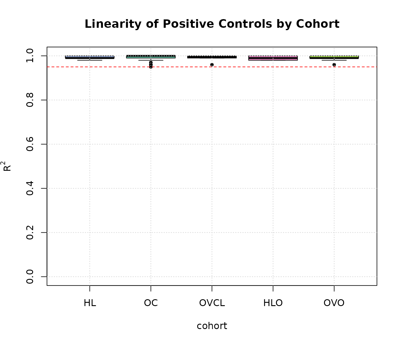
Plot of of positive control probes from samples across all cohorts.
Signal to Noise Ratio (SNR)
Level of Housekeeping Genes
boxplot(averageHK ~ cohort, ylab = "Average log HK expression",
        main = "Average log expression of Housekeeping genes by Cohort", data = expQC, pch = 20,
        col = c(COL.HLD, COL.OVD, COL.OVCL, COL.HLO, COL.OVO))
abline(h = 50, lty = 2, col = "red")
grid(NULL, NULL, lwd = 1)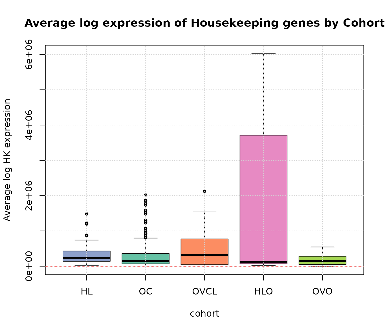
Average log expression of Housekeeping genes by Cohort.
Limit of Detection (LOD)
boxplot(lod ~ cohort, ylab = "LOD", main = "Limit of detection (LOD) by Cohort",
        data = expQC, pch = 20, col = c(COL.HLD, COL.OVD, COL.OVCL, COL.HLO, COL.OVO))
abline(h = 50, lty = 2, col = "red")
grid(NULL, NULL, lwd = 1)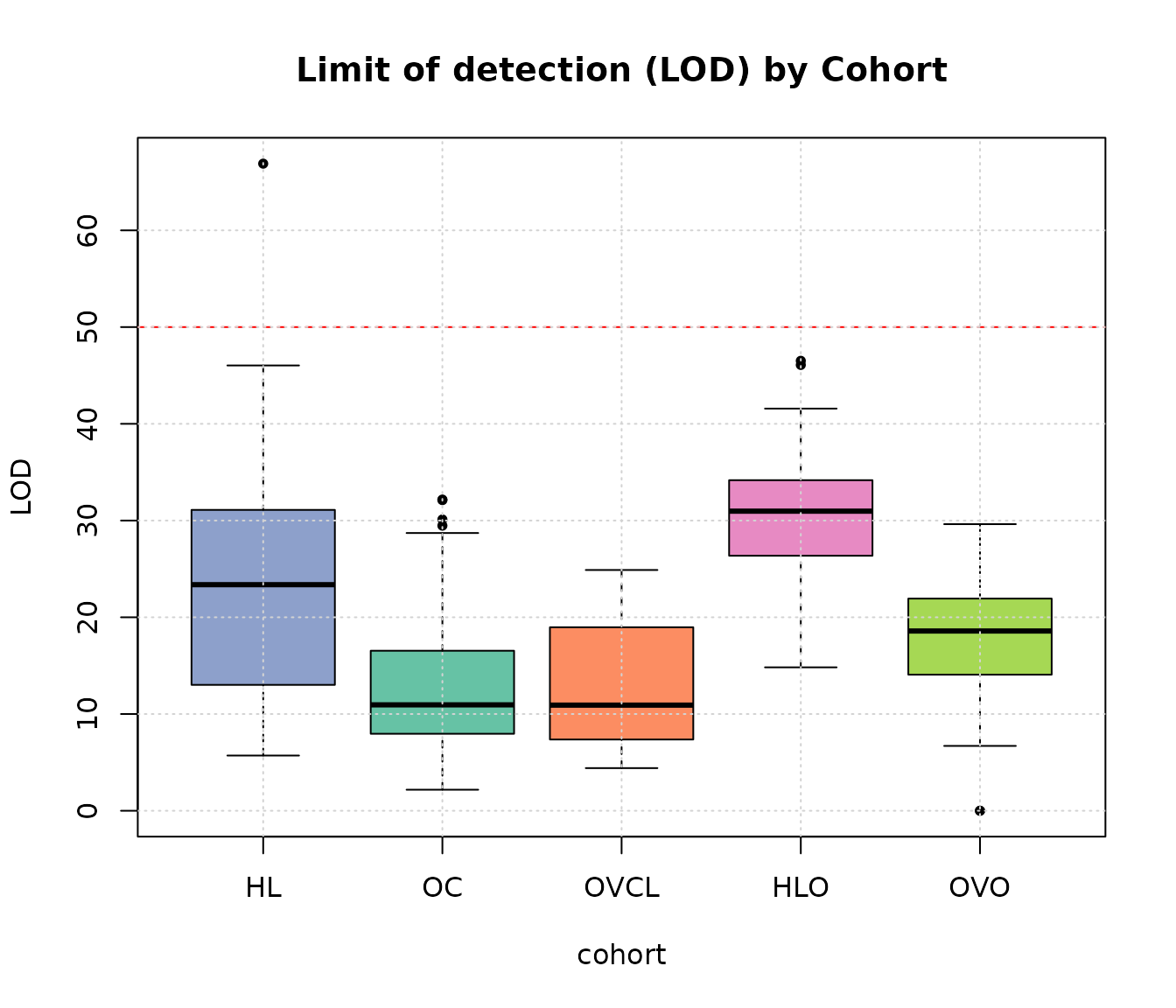
Limit of detection by cohort.
boxplot(pergd ~ cohort, data = expQC, border = "white",
       ylab = "% Genes Detected",
       main = "Percent of Genes Detected Above \n the Limit of Detection",
       pch = 20, col = c(COL.HLD, COL.OVD, COL.OVCL, COL.HLO, COL.OVO))
abline(h = 50, lty = 2, col = "red")
grid(NULL, NULL, lwd = 1)
stripchart(pergd ~ cohort, data = expQC,
           vertical = TRUE, method = "jitter",
           pch = 20, cex = 0.4 , col = "#3A6EE3",
add = TRUE) 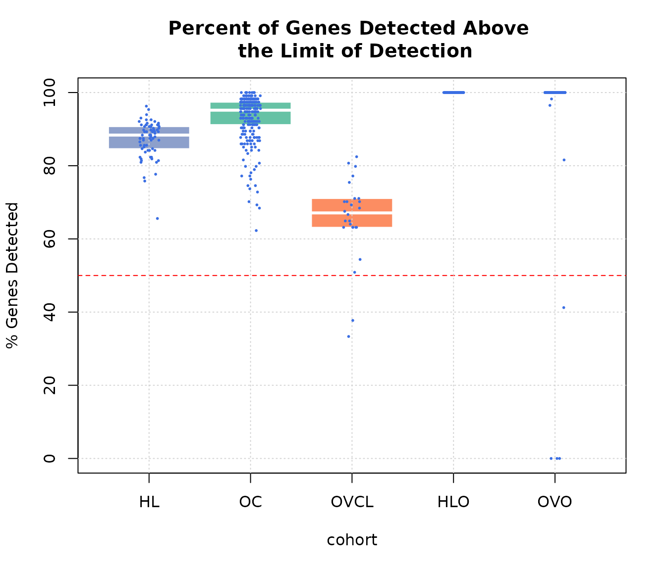
Percent genes of total (excluding controls) detected above the limit of detection.
sn <- 100
detect <- 60

plot(expOVD$sn, expOVD$pergd, pch = 20, col = COL.OVD, xaxt = "n", ylim = c(0, 100), xlim = range(expOVD$sn),
     xlab = "Signal to Noise Ratio", ylab = "% Genes Detected")
points(expOVO$sn, expOVO$pergd, pch = 20, col = COL.OVO)
points(expOVCL$sn, expOVCL$pergd, pch = 20, col = COL.OVCL)
points(expHLD$sn, expHLD$pergd, pch = 20, col = COL.HLD)
points(expHLO$sn, expHLO$pergd, pch = 20, col = COL.HLO)
axis(1, at = seq(0, max(expQC$sn) + 1, 300))
abline(v = sn, col = "red", lwd = 2)
abline(h = detect, lty = 2)
title("Signal to Noise vs \n Ratio of Genes Detected")
legend("bottomright", c("HL", "OC", "OVCL", "HLO", "OVO"), pch = 20, bty = 'n',
       col = c(COL.HLD, COL.OVD, COL.OVCL, COL.HLO, COL.OVO))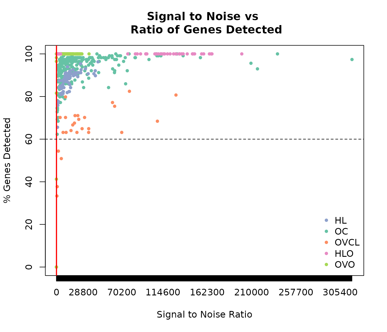
Signal to Noise versus % Gene Detected by cohort.
plot(expOVD$sn, expOVD$pergd, pch = 20, col = COL.OVD, xaxt = "n", ylim = c(0, 100), xlim = c(0, 6000),
     xlab = "Signal to Noise Ratio ", ylab = "Ratio of Genes Detected")
points(expOVO$sn, expOVO$pergd, pch = 20, col = COL.OVO)
points(expOVCL$sn, expOVCL$pergd, pch = 20, col = COL.OVCL)
points(expHLD$sn, expHLD$pergd, pch = 20, col = COL.HLD)
points(expHLO$sn, expHLO$pergd, pch = 20, col = COL.HLO)
axis(1, at = seq(0, max(expQC$sn) + 1, 300))

abline(v = sn, col = "red", lwd = 2)
abline(h = detect, lty = 2)
title("Signal to Noise vs \n Ratio of Genes Detected (Zooming-in)")
legend("bottomright", c("HL", "OC", "OVCL", "HLO", "OVO"), pch = 20, bty = 'n',
       col = c(COL.HLD, COL.OVD, COL.OVCL, COL.HLO, COL.OVO))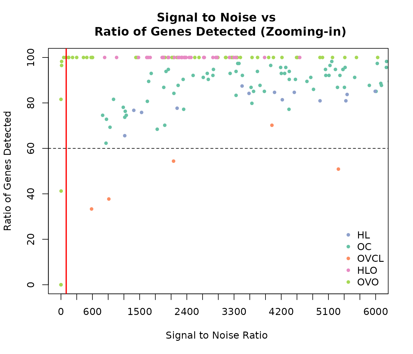
Signal to Noise versus % Gene Detected by cohort zoomed in to the area of possible failures.
HKnorm
The HKnorm function does a simple normalization to log transformed (base 2) gene expression data data to housekeeping genes. This is done by subtracting the average log housekeeping gene expression level from the expression level of every gene in each sample.
As an example, here we check the QC metrics of the Hodgkin Lymphoma data and normalize it to housekeeping genes:
We can check to see if any samples failed QC metrics
expHLD0 <- expHLD
any(expHLD0$QCFlag == "Failed")
[1] TRUE
expHLD0$sampleID[which(expHLD0$QCFlag == "Failed")][1] “HL1_3” “HL1_13” “HL1_17” “HL1_18” “HL2_3”
Since these are matched samples we must remove both pairs from the annotation data frame and from the gene expression data frame.
expHLD <- dplyr::filter(expHLD0, sampleID != "HL1_18" & sampleID != "HL2_18")
hld <- hld.r[, !colnames(hld.r) %in% c("HL1_18", "HL2_18")]
We now normalize the resulting gene expression data
# If data already log normalized
hld.n <- HKnorm(hld, is.logged = TRUE)

# Otherwise, normalize to HK
hld.n <- HKnorm(hld)
hld1 <- hld.n[, grep("HL1", colnames(hld.n))]
exp.hld1 <- subset(expHLD, geneRLF == "HL1")

hld2 <- hld.n[, grep("HL2", colnames(hld.n))]
exp.hld2 <- subset(expHLD, geneRLF == "HL2")
refMethod
This function does batch adjustment using a reference-based strategy.
Below is how this would work for the HL data:
r <- 3 # The number of references to use
choice.refs <- exp.hld1$sampleID[sample((1:dim(exp.hld1)[1]), r, replace = F)] # select reference samples randomly
R1 <- t(hld1[, choice.refs])
R2 <- t(hld2[, paste("HL2", getNum(choice.refs), sep = "_")])
Y <- t(hld2[, !colnames(hld2) %in% paste("HL2", getNum(choice.refs), sep = "_")])
S2.r <- t(refMethod(Y, R1, R2)) # Data from CodeSet 2 now calibrated for CodeSet 1
We can check the result by selecting a random gene and plotting the expression values from both CodeSets
set.seed(2016)
gene <- sample(1:nrow(hld1), 1)
par(mfrow = c(1, 2))
plot(t(hld1[gene, ]), t(hld2[gene, ]), xlab = "HL1", ylab = "HL2",
     main = "No Correction")
abline(0, 1)

plot(t(hld1[gene, !(colnames(hld1) %in% choice.refs)]), t(S2.r[gene, ]),
     xlab = "HL1", ylab = "HL2", main = "Corrected")
abline(0, 1)
HL1 vs HL2 gene expression with and without ccorrection